
Free-slip boundary conditions are used to simplify the physical behaviour at a domain boundary. It may be a free-surface where the boundary deforms slightly in response to the internal flow, or it may be an interface where the boundary layer thickness is so small that it cannot be resolved at the same time as the interior flow. The simplifying assumption: ignore the changes in shape, ignore the thin boundary layer, treat the surface as impenetrable, and the tangential stresses as vanishingly small.
In the weak form, boundary tractions appear as surface integrals. Multiplying the momentum balance by a test function and integrating by parts gives
Drop the surface integral and you have imposed zero traction in all directions — free everything (a free surface), not free slip. Constrain the surface-normal degrees of freedom and the surface integral only addresses the tangential traction terms.
On a Cartesian box, the first expression in (1) constrains a single velocity component. If we hold fixed on a vertical wall, the solver removes a row of unknowns, and there is no other work to be done. On a sphere, an annulus, any mesh that does not align with the coordinates, or a surface with topography, is not a single component of the unknown — it constrains a combination of unknowns at each point, and leaves other combinations free. That has the potential to make a simplifying assumption complicated to implement.
Let’s assume, for a moment, we confine ourselves to simple domains like the annulus, or a spherical shell, which are commonly used for planetary modelling. For each of these cases, there are coordinate systems, and well known forms of the differential operators that do restore the boundary condition to being a constraint in a single direction. Admittedly this requires reformulating all the equations, but for a symbolic-first code such as underworld, this is quite straightforward. This is the strategy used by CITCOMS Zhong et al, 2008. But not every domain boundary has a convenient coordinate system to follow. Even accounting for slight ellipticity introduces significant complexity in all the differential operators; anything more complicated will not have a useful coordinate reformulation.
The second condition in (1) is also worth noting. We don’t generally think about this when we constrain a degree of freedom, the other one/s, left unconstrained are natural to the problem. They fall out as traction-free surface conditions automatically in a finite element weak form. If we cannot simply eliminate one degree of freedom at each point, how do we satisfy all the parts of (1) ?
Four possibilities
We outline four possible approaches (all of which you can try out in Underworld3). They fall into two pairs: two impose the constraint weakly, by adding a term to the momentum equation and letting the solution satisfy the condition to within the accuracy of that term: a direct penalty, and Nitsche’s method, which differ in whether the term is consistent. Two impose it exactly: by construction, changing the basis so that the constraint is a component that can be struck out, or by a Lagrange multiplier, adding an equation that enforces it. The weak pair have a parameter to select that may need to be tuned for each problem and a floor they cannot go below. The exact pair are not tuneable, and they return the boundary traction as a side-effect of the solution. So does the direct penalty; Nitsche is the one that does not.
1. A direct penalty
This could not be more simple, conceptually. We are working in a variational environment, so we just add into our equation system, a term that punishes any flow through the boundary:
is a single scalar. It has to conform to the scale of the problem itself, which is why the value that works is a property of the model rather than a default.
One line, no new machinery, and it works on any geometry. What we are solving is a mildly perturbed problem and it is perturbed by exactly the amount the constraint cannot be satisfied: the discrete solution sits where the penalty term balances the boundary traction and this leaves small but not zero.
Making the residual smaller means pushing harder, and pushing harder degrades the condition-number of the operator. The error is traded against the conditioning, and (discussed below), this trade-off eventually stops returning any benefit.
Underworld codes this term it as a boundary traction opposing normal flow, using the surface normal at the quadrature points () provided by PETSc:
G = mesh.Gamma
penalty = 10000
stokes.add_natural_bc(penalty * G.dot(v.sym) * G, "Upper")
The topography is the penalty term itself. That term is the traction the condition holds the wall with, so on the boundary
which is arithmetic on values the solve already returned — nothing is differentiated and nothing is solved.
n = mesh.boundary_normal("Upper")
sigma_nn = -penalty * n.dot(v.sym)
That is a saving in cost and not in accuracy. The leak and the traction are the same quantity scaled by , so a coefficient too small to hold the boundary reports a traction that is short in the same proportion.
Nitsche’s method
The reason the penalty is only accurate in the limit is that it is not consistent: substituting the true solution does not fully satisfy the equation, because the true solution is subject to a separate boundary traction the penalty form ignores. Nitsche’s method 2 restores consistency by carrying that traction explicitly:
The first of the three is the consistency term: it is the boundary traction the integration by parts produced, and including this makes the true solution satisfy the discrete equations exactly. The second is its transpose, which keeps the form symmetric and buys optimal convergence in . The third is the penalty again, and it is still needed — but now for stability rather than for accuracy, and has a threshold set by an inverse inequality rather than being an unspecified free parameter.
This is a real improvement and it is still done through a weak imposition. The constraint holds to the accuracy of the discretisation, not to the accuracy of the arithmetic — measured below, it leaks a few parts in a thousand on a typical mesh, and the leak falls with increasing mesh resolution.
The topography has to be recovered from the solved fields, which is where Nitsche parts company with the direct penalty. Its boundary term is the penalty part less the consistency terms, and those are written in , so the traction cannot be read off without differentiating the velocity. Recover that way and divide by .
A constraint equation, with a multiplier
The two strategies above add a term to the weak form of the equation. This approach adds an equation.
Carry a scalar field on the boundary and require, as a row of the system in its own right,
where is the prescribed wall-normal velocity — zero for free slip, and a datum if the wall is being driven — and enters the momentum row as the traction that holds the constraint. It is a Lagrange multiplier, and the system becomes a larger saddle point: velocity, pressure, and now .
has units of stress. At convergence it is on that boundary, so dividing by (density contrast gravity) is the dynamic topography.
The constraint row is exact, so unlike a penalty there is no parameter whose size decides how well it holds. Two practical things do have to be dealt with.
is carried as a full-domain field but only its boundary trace means anything, so the interior degrees of freedom are constrained out of the global system in the section before the solve sees it. They are not solved for and are not stored in the block.
The Schur complement is poorly conditioned on its own, so an augmented-Lagrangian term is added to the momentum row. It does not change what the constraint enforces, because the row still carries the exact constraint.
stokes = uw.systems.Stokes_Constrained(mesh, velocityField=v, pressureField=p)
lam = stokes.add_constraint_bc(0.0, "Upper")
stokes.solve()
The Stokes_Constrained solver carries three fields in PETSc — velocity, pressure and — and splits them two ways: velocity against the pair, with the volume constraint (incompressibility) and the boundary constraint grouped into a single Schur block. The boundary constraint applies to surface nodes only.
That boundary term is the whole boundary load, , not the multiplier alone. The second part vanishes only where the constraint row is satisfied exactly; discretely it is satisfied to the solver’s tolerance, and multiplies that residual back into the traction. With a viscosity-weighted and a lateral viscosity contrast it can be the largest term of the result, so the two parts are not separable in practice.
Rotating the degrees of freedom
In this approach, we stop “asking for” the constraint and just impose it. At each constrained node, we change the coordinate basis in which the velocity unknowns are expressed, from the global Cartesian frame to the local frame. In that basis “no flow through the boundary” is again a single component, and it is removed the same way it would be on a box.
Collect the per-node rotations into a block-diagonal , equal to the identity at every node that is not constrained. The rotated system is
and the wall-normal row of is struck out. The constraint then holds to machine precision, because it is not being solved for at all.
This is the classical strategy. It is found in the early finite-element literature, for example Engelman, Sani and Gresho 3 reviewed the alternatives and chose between them on grounds of global mass conservation. What is worth understanding is why, given that it is exact and the others are not, it is the least used of the three.
The topography is the reaction of that struck row — the force the constraint had to supply — de-smeared by the boundary mass to turn an integrated nodal load into a pointwise stress,
which is the consistent boundary flux of Zhong, Gurnis and Hulbert 4. In Underworld3, the solver’s boundary_normal_traction() and dynamic_topography() return these. Nothing is differentiated and nothing is solved: in two dimensions is lumped and the de-smear is a division.
Trade-offs
Rotating the degrees of freedom leaves the discrete problem in a mixed basis. Interior nodes hold ; constrained nodes hold . Nothing about that is difficult in itself, but everything downstream has to agree about which nodes are which.
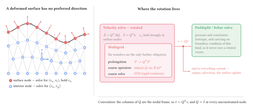
Where the rotation lives. The obligation is contained: the velocity solve is rotated and carries its multigrid with it, while the Schur complement and the pressure solve beside it never handle a rotated vector, because the pressure block carries no boundary condition of this kind. One un-rotation sits on the boundary between them and feeds both.
Four objects carry : the operator, the right-hand side, the solution on the way out, and the multigrid prolongation. The coarse operators inherit it through the Galerkin triple product rather than being rotated separately, and the coarse solve should be an SVD, because a Galerkin-coarsened rotated operator inherits any rigid-rotation null space of the constrained problem (the exact constraint makes the null space of the sphere and the annulus a dominant feature of the solve).
We do not know the cost of the addtional complexity on the solver and setup times, or on the accuracy of the solution but this can be measured and will differ from problem to problem.
Choice of the surface normal
In a discrete representation of a curved surface, the normal can be defined in various ways. The boundary of a discretised domain is a set of straight facets, and the assembled constraint is an integral over those facets. The node normal consistent with that integral is the average of the adjacent facet normals weighted by facet measure — not the normal of the smooth surface the mesh approximates, and not the facet normal on its own.This is the consistent normal of Engelman, Sani and Gresho 3. They derived this result in 1982 from global conservation of mass.
The analytic normal is exact for the geometry and therefore inconsistent with the discretisation: the solver is not solving on the sphere (or annulus), it is solving on the polyhedral approximation to the sphere.
Using the facet normal is worse than inconsistent, it can prevent us obtaining a solution. In 2D, imposing facet by facet requires a node shared by two facets to satisfy two different constraints, and two independent constraints on a two-component velocity provide no freedom. Push the penalty higher, and the vertex velocities go to zero: the flow is being asked to stay inside a polygon rather than a circle, and the discrete limit is a different problem from the smooth one. Refining the mesh does not fix this — the velocity error does not approach zero (python3 stress.py locking).
On an annulus with a free slip boundary, the direct-penalty approach locks at high penalty values () if facet normals are used in the constraint equation. In the figure below, the node-normal approach does solve and reproduces the analytic solution (described in detail in the next section)
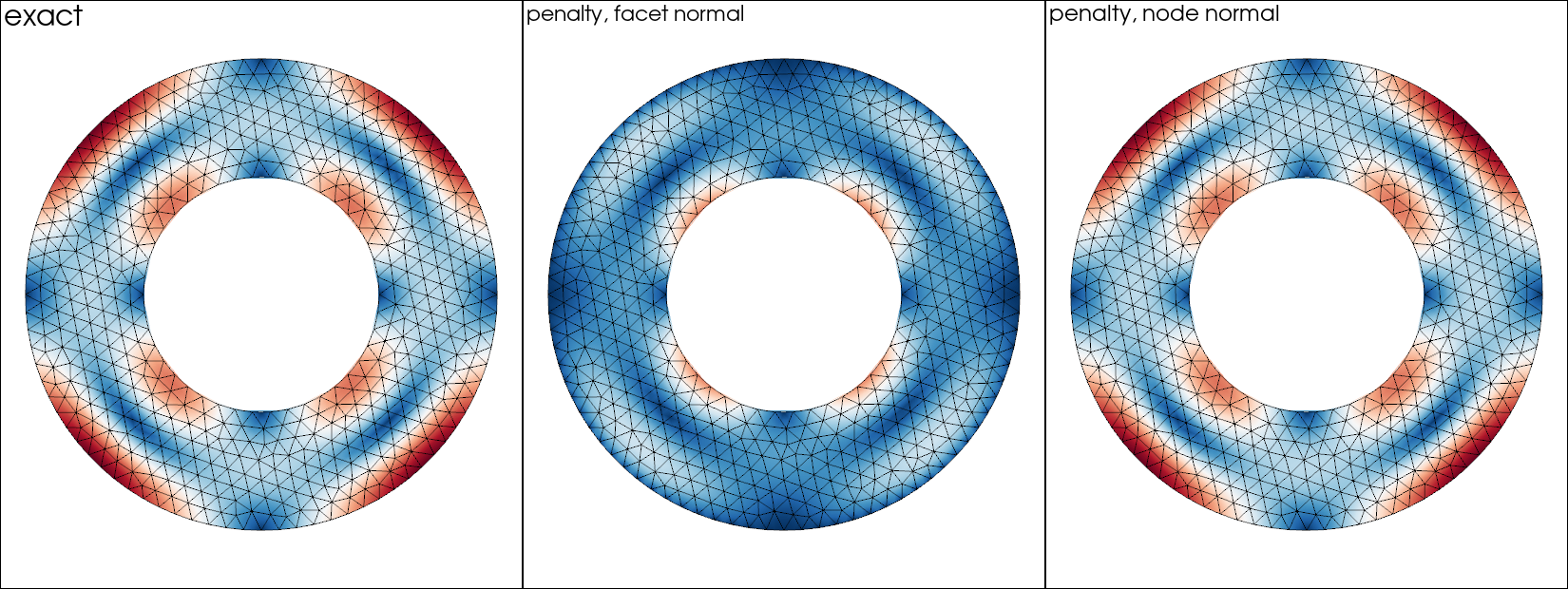
The same problem, the same penalty and the same scale: against the facet normal the flow along the outer boundary is suppressed — the peak speed falls by a quarter and the two fast lobes at the boundary are gone. Against the measure-weighted node normal it matches the exact solution to plotting accuracy at this resolution.
Everything that follows uses the node normal, which is what add_nitsche_bc and add_rotated_freeslip_bc take by default and what mesh.boundary_normal returns. The facet normal does not appear again.
When the choice of constraint matters
Solve a convection model with any of these approaches, and the velocity field is the same to plotting accuracy. Generally speaking, a leak of order 10-3 or 10-4 in is within the expected accuracy of the solution on the mesh and the main driver of which method to choose should be solver efficiency (wall time).
The difference in the methods appears when the wall-normal traction is a required output of the model: dynamic topography, geoid, gravity, or a plate-boundary force balance require accurate integration of boundary stresses. Here the choice becomes more subtle, and the methods have quite different accuracies, and different efficiencies.
The benchmark
Kramer, Davies and Wilson 5 give exact Stokes solutions in a cylindrical annulus, and their assess package publishes the radial stress as well as the velocity, which is what makes it an oracle for this question rather than only for the flow. Underworld wraps it as uw.analytic.CylindricalStokes.
The case used throughout is the smooth one: a density anomaly with and , viscosity 1, free slip on both radii. On the outer boundary the exact radial stress is a single harmonic,
fitted to a residual of 10-16, so the whole of the surface stress is that one amplitude and the error in it is one number. The treatment under test is on the outer radius; the inner carries the exact analytic velocity as a Dirichlet condition, so it is the only free-slip condition in the model.
Two things are measured on every solve:
the surface permeability — the largest on the outer boundary, against the true radial direction, divided by the flow speed. The fraction of the flow going through an impermeable boundary.
the boundary stress error — the relative error in that harmonic amplitude, recovered from the solved fields by projection, which is the route every method has available.
Penalty at , Nitsche at .
| cell size | penalty | Nitsche | multiplier | rotated |
|---|---|---|---|---|
| 0.150 | 3.1 × 10⁻³ / 2.5 × 10⁻² | 1.0 × 10⁻² / 5.8 × 10⁻² | 2.3 × 10⁻⁴ / 2.4 × 10⁻² | 5.3 × 10⁻¹¹ / 2.4 × 10⁻² |
| 0.100 | 3.0 × 10⁻³ / 1.1 × 10⁻² | 2.4 × 10⁻³ / 2.4 × 10⁻² | 1.0 × 10⁻⁴ / 1.0 × 10⁻² | 5.8 × 10⁻¹¹ / 1.0 × 10⁻² |
| 0.075 | 3.0 × 10⁻³ / 7.2 × 10⁻³ | 1.2 × 10⁻³ / 1.5 × 10⁻² | 8.6 × 10⁻⁵ / 6.3 × 10⁻³ | 1.2 × 10⁻¹⁰ / 6.2 × 10⁻³ |
| 0.050 | 3.0 × 10⁻³ / 3.6 × 10⁻³ | 2.7 × 10⁻⁴ / 6.3 × 10⁻³ | 6.7 × 10⁻⁵ / 2.7 × 10⁻³ | 1.2 × 10⁻¹⁰ / 2.7 × 10⁻³ |
Reading the leak first, Nitsche leaks parts in a thousand and improves with the mesh — the rate consistency buys. The multiplier is an order of magnitude better and improves faster. The rotated constraint does not move: it sits at the solver’s floor at every resolution, because the mesh has nothing to do with it. The penalty does not improve either, and for the opposite reason — its leak is set by the penalty coefficient rather than by the discretisation.
Reading the stress column, the ranking changes. Every treatment that imposes the constraint correctly lands on the same stress error at a given mesh: 6.3 × 10⁻³ for the multiplier and 6.2 × 10⁻³ for the rotated constraint at cell 0.075, where their leaks differ by nine orders of magnitude. What sets that number is the recovery — a projection of a stress differentiated out of a piecewise-quadratic velocity — and not the boundary condition underneath it. A constraint held to 10-10 buys nothing over one held to 10-4 if the answer is then recovered the same way.
Nitsche is the exception, at twice the error of the others on the coarser meshes. Its is enough for the leak and not for the stress: at the leak improves by a factor of nearly forty and the stress by a factor of two, onto the same floor as everything else, after which more buys nothing.
Traction extraction v. Stress recovery
Three of the four treatments do not have to recover anything. The two exact ones carry the traction as a constraint reaction or as an unknown, and the direct penalty carries it as the term it adds. Against the same exact answer:
| cell size | rotated, reaction | multiplier, traction | penalty, | recovered by projection |
|---|---|---|---|---|
| 0.150 | 6.8 × 10⁻³ | 8.6 × 10⁻³ | 9.0 × 10⁻³ | 2.4 × 10⁻² |
| 0.100 | 3.3 × 10⁻³ | 8.5 × 10⁻⁴ | 1.2 × 10⁻³ | 1.0 × 10⁻² |
| 0.075 | 2.1 × 10⁻³ | 1.7 × 10⁻³ | 2.3 × 10⁻³ | 6.3 × 10⁻³ |
| 0.050 | 1.1 × 10⁻³ | 1.4 × 10⁻³ | 2.2 × 10⁻³ | 2.7 × 10⁻³ |
Better than the projection on the same solve at every resolution, using the expressions given with each method above — by an order of magnitude at best, and by very little where the penalty’s coefficient sets its floor. None of the three falls smoothly with : part of what they report is the constraint residual, and how low a particular solve can drive that is not a function of the mesh. For the penalty that is the whole story below a cell size of 0.1 — its leak is 3 × 10⁻³ at every resolution here, set by , and the traction it reports cannot be better than its ability to satisfy the constraint.
Influence of penalty parameters
The two weak methods look alike in the comparison above, but this is for a fixed, tuned penalty parameter.
| (penalty) | leak | (Nitsche) | leak | |
|---|---|---|---|---|
| 10² | 2.6 × 10⁻¹ | 1 | diverged | |
| 10³ | 2.6 × 10⁻² | 10 | 1.7 × 10⁻³ | |
| 10⁴ | 2.6 × 10⁻³ | 100 | 2.7 × 10⁻⁴ | |
| 10⁵ | 3.0 × 10⁻⁴ | 1000 | 3.0 × 10⁻⁵ | |
| 10⁶ | 4.5 × 10⁻⁵ | 10⁴ and above | diverged |
Nitsche is bounded at both ends. Below the form is no longer coercive and no amount of solver tuning recovers a solution; from in this problem, the line search stops converging. The virtue of is that it sits within that window on any mesh, because is dimensionless and the term it scales already carries .
The penalty coefficient scales differently because it directly penalises the value of the velocity across the boundary. It should therefore scale with the characteristic velocity which is best estimated from the magnitude of the forcing terms and the resisting viscosity.
Written against the node normal, the penalty simply trades: a decade of coefficient for a decade of leak, all the way to 106, with no wall in this problem. What it does not do is converge with resolution — the leak is bought with the parameter rather than with the mesh resolution — so the coefficient has to be re-chosen whenever the forcing or the viscosity changes.
Multiplier and CBF equivalence
The two expressions given above for computing topography from the boundary reaction are exactly equivalent. Write the momentum row’s boundary term out and the identity is immediate: the assembled load is , and at convergence it balances the volume residual restricted to the boundary, which is precisely the nodal load the consistent boundary flux back-calculation reads 4. So
which is the rotated constraint’s reaction, de-smeared with the same boundary mass. The multiplier is not an independent estimate of the surface stress: it is the same computation, arrived at by carrying the traction as an unknown instead of reading it out of the residual afterwards.
Lateral viscosity contrast case
No published solution has both a curved boundary and a laterally varying viscosity, so the case where weak constraints are most often reported to give trouble is a separate test with a simple geometry. SolCx is a good example: unit box, free slip on all four walls, viscosity 1 to the left of and to the right. uw.analytic.SolCx publishes the exact dynamic topography on the top wall. Three walls carry the ordinary component condition and the treatment under test is on the top wall alone.
On a box every treatment reduces to holding one velocity component. What it can say is whether a treatment holds the traction it was given when the viscosity beside it jumps. However, on a box the rotated constraint’s per-node rotation is the identity, so the table below exercises none of the rotation machinery. We check that separately on an equivalent problem: the domain, the gravity vector and the exact solution all turned by 45°, with every wall then carrying the rotated constraint, because a component condition cannot express on a tilted wall. Turned, the constraint still holds to machine precision and the velocity error is unchanged at 8.8 × 10⁻⁶; imposing the un-turned condition on those same walls instead lets 71% of the flow through the boundary.
In the table below, we show the relative error of the surface topography along the top wall, mean removed, at 32 × 32 elements. Each entry is the whole wall and then the wall with two elements trimmed from each end.
| component Dirichlet | penalty, 104 | multiplier | rotated | |
|---|---|---|---|---|
| 10 | 0.048 / 0.054 | 0.045 / 0.051 | 0.048 / 0.054 | 0.048 / 0.054 |
| 10² | 0.072 / 0.081 | 0.056 / 0.060 | 0.072 / 0.081 | 0.072 / 0.081 |
| 10³ | 0.075 / 0.084 | 0.234 / 0.230 | 0.075 / 0.084 | 0.075 / 0.084 |
| 10⁴ | 0.076 / 0.085 | 0.698 / 0.697 | 0.076 / 0.085 | 0.076 / 0.085 |
| 10⁶ | 0.076 / 0.085 | 0.992 / 1.000 | 0.075 / 0.084 | 0.076 / 0.085 |
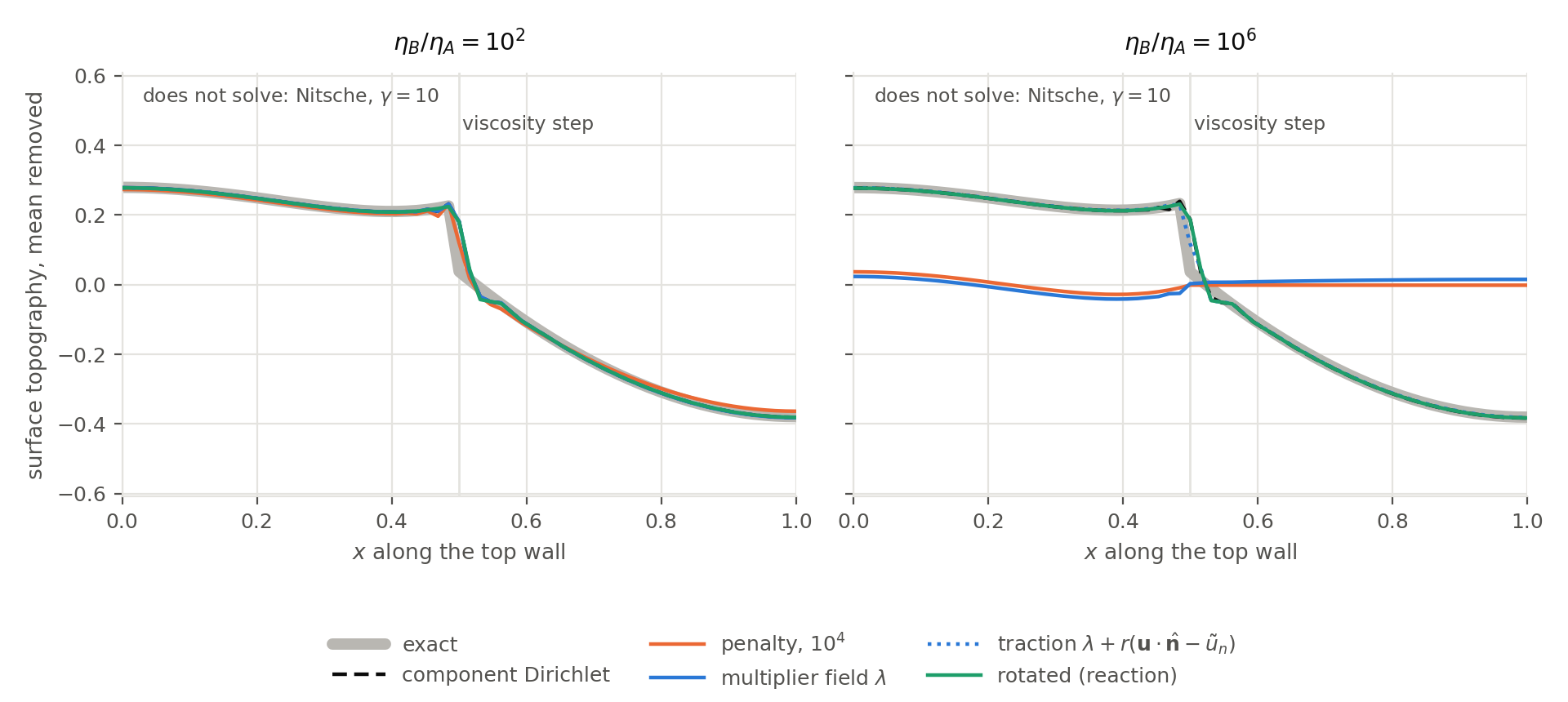
Surface topography along the top wall, against the exact answer. At a contrast of
100 nothing distinguishes the treatments. At 106 the multiplier field
carries almost none of the traction on its own — the augmentation
holds the rest — while , which is what traction() returns, lies on the exact curve. The
penalty has failed by this contrast: its coefficient is a bare number and cannot
be large against 106 and moderate against 1 at the same time.
The three exact treatments agree to three figures at every contrast, whole wall and trimmed alike. That is the result to take from this half, and it took the multiplier reporting the whole traction rather than alone, and the rotated constraint holding the corner where it meets the side walls.
Read the first column as the reference. The component Dirichlet condition is exact and has no parameter, and its velocity error is 8.8 × 10⁻⁶ at a contrast of 106. It still reads 0.085. That number is the recovery’s error, not a boundary condition’s: on the stiff half the recovered is a difference between the pressure and with , so a relative velocity error of 10-5 appears in the stress.
A bare penalty coefficient cannot serve both halves. At 104 it is the best column in the table at low contrast (the constraint is weak enough not to fight the recovery) but by 106 it is meaningless: 0.992, which is to say the recovered topography carries none of the signal. Reading instead of recovering the stress gives the same numbers to three figures, here and at every coefficient tried, which is the point made above from the other side: the term is the traction, so it inherits the error in the constraint rather than curing it. Scaling the coefficient by the local viscosity is the obviously right thing to want, but the solver does not converge here at any magnitude we tried, from to .
Nitsche has no column in this table. In our implementation it is unreliable on a boundary that mixes essential patches with Nitsche patches, which is what this test asks for: the top wall weak, the other three held strongly. We could not reach a converged solution for this example at any penalty. Imposed weakly on all four walls does converge, but that is a different problem.
Solver timing
Seconds on the annulus, uniform viscosity, one core, direct solver: the solve, and then the surface traction by whatever route that treatment has. Median of three timed repeats after an untimed warm-up, run sequentially. Two sizes, because below about ten thousand nodes the four are separated by less than the run-to-run spread and there is nothing to read.
| velocity nodes | penalty | Nitsche | multiplier | rotated |
|---|---|---|---|---|
| 28 338 | 0.17 / — | 0.18 / 0.267 | 0.26 / — | 0.16 / 0.010 |
| 71 424 | 0.45 / — | 0.47 / 0.657 | 0.67 / — | 0.43 / 0.016 |
The dash indicates that the multiplier and the penalty do not require any additional solver — is a finite element field in its own right, so its nodal values are the traction, pointwise, and is an expression evaluated where it is wanted. The penalty traction is recovered similarly as the penalty scaling the leakage velocity.
The rotated constraint’s reaction does need one step. The reaction is an integrated nodal load, , which is times the pointwise traction. Turning it into a pointwise value means undoing that boundary mass. On a 2-D trace, and on 3-D P1 triangles, the lumped mass is diagonal and undoing it is a division — the 10 to 16 ms above. On 3-D P2 triangles it is a true solve: the lumped row sums vanish at the vertices, so the consistent trace mass has to be assembled and solved. That is the one place the CBF route pays for being a back-calculation.
The multiplier’s solve costs about 50% more, consistently — 0.67 s against 0.43 s at 71 000 nodes. That is the extra field and the larger saddle point. Rotating the degrees of freedom costs nothing measurable against the weak forms: the rotation is a sparse orthogonal transform on a boundary’s worth of rows.
Nitsche has to recover surface stress by differentiating the solution, and the projection that does it costs more than the Stokes solve did — 0.63 s against 0.45 s — so asking a Nitsche model for its surface stress roughly doubles the timestep. The direct penalty need not pay that: its own term is the traction, read as arithmetic on the boundary nodes.
The obvious question is whether that is the method’s cost or the recovery’s. A global projection to get values on a thousand boundary nodes is plainly more work than the job requires, and the consistent boundary flux is a viable alternative, reading the assembled residual rather than differentiating anything. However, we find that it does not work for a weakly imposed condition, and the reason is the same one that makes it unavailable to the multiplier:
| cell 0.0125 | projection | CBF back-calculation |
|---|---|---|
| penalty, node normal | 0.651 s, error 1.1 × 10⁻³ | 0.224 s, error 1.00 |
| Nitsche | 0.666 s, error 3.6 × 10⁻⁴ | 0.230 s, error 1.00 |
| rotated | 0.602 s, error 1.6 × 10⁻⁴ | 0.206 s, error 1.6 × 10⁻⁴ |
An error of 1.00 just means that no topography was recovered. With the weak constraint, the boundary stress is recovered using the multiplier . In the penalty case, the boundary traction is . Nitsche’s term is written in terms of , so reading it back still requires differentiating the answer.
That is the structural point inherent in the timing table and it follows the pairing of the strategies:
| how the constraint is imposed | the traction is | to read it |
|---|---|---|
| weakly, by a penalty term | the term itself | evaluate |
| weakly, by Nitsche | inside a term written in | differentiate the solution |
| exactly, by construction (rotated) | the constraint reaction | de-smear the nodal load |
| exactly, by a multiplier | an unknown of the system | read the field |
Which one to use
For a model that consumes the velocity and nothing else, all four are the same to plotting accuracy — provided the constraint is written against the node normal. That proviso is the only one that can spoil the velocity, and it costs one line.
When the wall-normal traction is needed:
Rotated free slip is the default. It holds the constraint to machine precision rather than to the discretisation, its reaction is the most accurate surface stress measured here, and that reaction is nearly free. The price is structural — a mixed basis that the multigrid has to carry — and it is paid once, inside the solver, rather than by the person setting up the model.
The multiplier is its equal on accuracy and returns the same object by a different route; take it when you want the traction as an unknown of the system, or when the constrained problem’s conditioning suits you better. It costs about 50% more to solve.
Nitsche is the one to reach for when the boundary condition must change during the model — a wall that begins as a prescribed velocity and relaxes to a prescribed traction is a Nitsche problem, because a hard constraint cannot morph. Budget for tuning against the stress and not against the leak, and expect the window to move with the viscosity contrast. If the viscosity contrast is large with jumps or strong gradients along the boundary, be very careful if you choose Nitsche.
A direct penalty is fine for a velocity-only model and needs the node normal, a coefficient chosen per problem, and a check on something physical before the answer is believed. It will also hand back the traction it holds the wall with, at no cost, and that reading is worth no more than the coefficient behind it. It has the advantage that this is pure, direct penalty on the weak form and can be used for many things beyond simply boundary conditions. Good for a first pass on a very general idea.
Using it
import underworld3 as uw

mesh = uw.meshing.Annulus(radiusInner=0.5, radiusOuter=1.0, cellSize=0.05)
stokes = uw.systems.Stokes(mesh)

# Value first: 0 is free slip. A non-zero scalar or expression prescribes the
# wall-normal datum u.n = u_n strongly instead.
stokes.add_rotated_freeslip_bc(0.0, "Upper")
stokes.add_rotated_freeslip_bc(0.0, "Lower")

stokes.solve()

# The constraint reaction, which is the boundary normal traction.
sigma_nn = stokes.boundary_normal_traction("Upper")
Leave the normal to Underworld unless the constraint has to follow the true surface rather than the mesh. Passing an analytic normal — X / |X| on a sphere — is exact for the geometry and keeps a consistency error against the faceted assembly, which is usually not what you want.
Reach for Nitsche when the boundary condition has to change during the model. A hard constraint cannot morph: a wall that begins as a prescribed velocity and relaxes to a prescribed traction is a Nitsche problem, because the rotated constraint is either imposed or it is not.
- Zhong, S., McNamara, A., Tan, E., Moresi, L., & Gurnis, M. (2008). A benchmark study on mantle convection in a 3‐D spherical shell using CitcomS. Geochemistry, Geophysics, Geosystems, 9(10). 10.1029/2008gc002048
- Nitsche, J. (1971). Über ein Variationsprinzip zur Lösung von Dirichlet-Problemen bei Verwendung von Teilräumen, die keinen Randbedingungen unterworfen sind. Abhandlungen Aus Dem Mathematischen Seminar Der Universität Hamburg, 36(1), 9–15. 10.1007/bf02995904
- Engelman, M. S., Sani, R. L., & Gresho, P. M. (1982). The implementation of normal and/or tangential boundary conditions in finite element codes for incompressible fluid flow. International Journal for Numerical Methods in Fluids, 2(3), 225–238. 10.1002/fld.1650020302
- Zhong, S., Gurnis, M., & Hulbert, G. (1993). Accurate determination of surface normal stress in viscous flow from a consistent boundary flux method. Physics of the Earth and Planetary Interiors, 78(1–2), 1–8. 10.1016/0031-9201(93)90078-n
- Kramer, S. C., Davies, D. R., & Wilson, C. R. (2021). Analytical solutions for mantle flow in cylindrical and spherical shells. Geoscientific Model Development, 14(4), 1899–1919. 10.5194/gmd-14-1899-2021