Faults can dominate the dynamic behaviour of Earth systems at scales from the entire planet to a few 10s of metres. They are an extreme example of localisation: feedback between forcing and response that results in self-reinforcing weakening that does not have a brake at the largest scale. Faults are extreme in the sense that their natural thickness is orders of magnitude below that of a typical tectonic simulation.
At the tectonic scale, a fault is an infinitesimally thin surface across which the rock moves discontinuously by overcoming a frictional resistance. A finite element mesh (the mesh we use in Underworld) is a mechanism for representing continuous fields and there is not a native mechanism that perfectly represents a fault.
There are lots of different potential solutions to this difficulty. They include: 1) ignoring it by using a continuum model of the fault, 2) adding extra interpolation functions that represent discontinuities, 3) splitting the mesh along the line of the fault and dealing with it as a surface, 4) refining the mesh enough that the fault width is invisibly small at the model length scale.
Faults in numerical models
Localisation is something a rheological law produces all by itself: if we give the material a yield stress or a strain-rate-weakening viscosity, shear bands appear where the stress requires them, with an orientation determined by the stress, and at whatever width the physics and the mesh between them allow. Do we really need to do anything more than this to represent faults ? The answer is yes and there are two main reasons.
First, a fault is not in the same category as a shear band or a damage-zone. At the lithospheric scale a fault is persistent through changes in the tectonic loading. Faults localise far more sharply than any band a lithosphere-scale mesh resolves, down to a gouge zone of metres or even less. They are self-reinforcing: once a fault has accumulated slip it has juxtaposed distinct rock units; the weakness becomes structural and persistent even when the load is absent. Faults have history.
Second, conceptually, at the tectonic scale fault is an infinitesimally thin surface across which the rock moves discontinuously by overcoming a frictional resistance. A finite element mesh (the mesh we use in Underworld) is a mechanism for representing continuous fields and there is not a native mechanism that perfectly represents a fault. Faults are sub-grid objects with their own constitutive properties.
That is why it is common to impose plate boundaries in a mantle model as prior knowledge 1, and why those plate boundaries often have additional evolution rules.
It is also why crustal models of stress build-up and release always try to include known faults. They are very fine-scale structures, they reflect complex geological history and they are not simply emergent from the imposed loading.
Describe the fault not the implementation
The fault geometry and its numerical representation ought to be decoupled as far as possible. It is the thesis of both Zhong & Gurnis (1995) and Sandiford & Moresi (2019): what the fault surface is, and what the solver is asked to do with it, are distinct choices. The first is a statement about the Earth: this is the fault surface, sampled as a polyline in two dimensions or a triangulated sheet in three, curved as it likes. The second is a modelling choice: this surface is to become a slippery interface, or a weak band of a stated width, or a direction of easy shear painted into the rheology. The same surface supports all of them and is agnostic to the implementation.
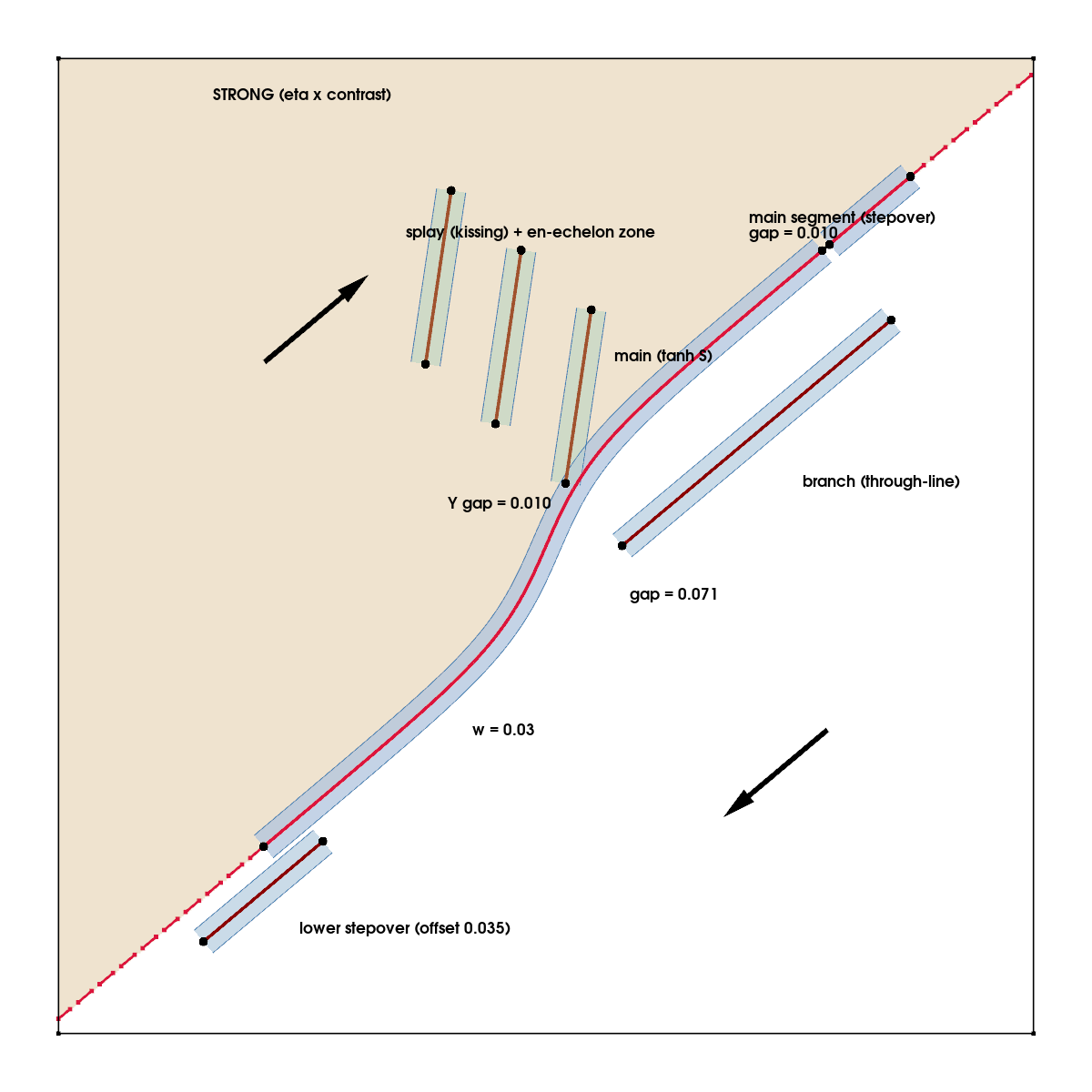
Figure 1:A synthetic fault network that we use to validate the different fault algorithms.
Figure 1 shows a synthetic fault network for our 2D and 3D experiments. The network is described by a number of independently meshed vertical segments in 3D and their surface traces for 2D models. It has a number of characteristics designed to test the fault implementation: multiple faults in a single domain; curved faults; junctions; steps and segment breaks for a single fault. There is a material property jump across the main fault in this network. The system is driven by boundary shear.
Three implementations
There is no perfect choice in how we model a fault in a geodynamic context and that means keeping several possible choices on hand to see which one works best for a specific problem. Underworld3 offers three: a weak zone, a weak zone with a direction, and a cut. Each of them can be built on the unstructured mesh, or on a mesh modified to conform to the fault.
| Mesh untouched | Mesh conforms to the fault | |
|---|---|---|
| Weak zone | painted band — the mesh sets the width | ribbon — the width is prescribed |
| TI weak zone () | painted, director from the distance gradient | TI ribbon — the width is prescribed |
| Cut | XFEM: enrichment functions carry the jump through the elements (not in Underworld) | split nodes with additional degrees of freedom |
The non-conforming, transversely isotropic (TI) rheology requires no changes to the mesh to represent the mechanics of the fault. It simply creates a near-fault band of material that has a lower frictional strength parallel to the fault: the material there resists shear on the fault plane with a second, smaller viscosity , and everything else with the background viscosity . There is a zone of weakness that depends on the perpendicular distance to the fault object, and the internal orientation is given by the perpendicular vector to the fault surface. The band is whichever cells fall within of the fault, so its width is set by the mesh as much as by . The resulting zone of weakness crosses element boundaries and can produce anomalous stress concentrations along the fault. These are mitigated at the large scale by refining the triangulation and smoothing the fault’s influence function but they never disappear 4. This is the representation of Sharples et al. (2015) and of Sandiford & Moresi (2019).
Material property jumps can be incorporated into finite element representations when they lie along element boundaries. It is therefore possible to represent a fault as a rheologically distinct volume if we are prepared to remesh. The weak ribbon is a band of width meshed along the fault trace — its vertices are the fault’s own points offset by either side — with a contrasting rheology in that region (a weak zone, or a zone with its own plasticity coefficients). For this we do need the ability to remesh so it is more difficult to implement in models where the fault system evolves. In this model, the fault, as a volume under normal stress, can deform internally and violate the frictional surface approximation. This is primarily an issue when is significantly larger than the fault’s true physical width.
The latter problem can be alleviated by combining the first two approaches. A TI ribbon is the same band but using the transversely isotropic frictional model of Moresi & Mühlhaus (2006) within the remeshed band: the same rheology as the non-conforming case, with the remesh taking control of the width. This has the same desirable properties from the finite element solver’s point of view as the weak band model, but it can transmit normal stresses across the fault without internal flow.
The split algorithm is the one that embraces the notion of the fault as an embedded surface. It produces a cut through the mesh to create a new internal surface boundary. In general this is also a remeshing step: the mesh is cut along the fault line, dividing the elements it crosses, and degrees of freedom are added along the cut; Zhong & Gurnis (1995) put slippery nodes into a convection model this way, on a hexahedral grid nudged towards the fault. We make the mesh conform to the fault beforehand, so that what remains is the duplication alone. Faults are surfaces that conform to element boundaries but they are implemented as pairs of surfaces to represent the two sides of the fault. The constitutive model lies in the interaction of these two coincident surfaces. This is a good choice of model when the physical scale completely precludes resolving , but there are some limitations: because the mesh is cut into sliding surfaces, there are incompatible constraints when two faults meet or cross.
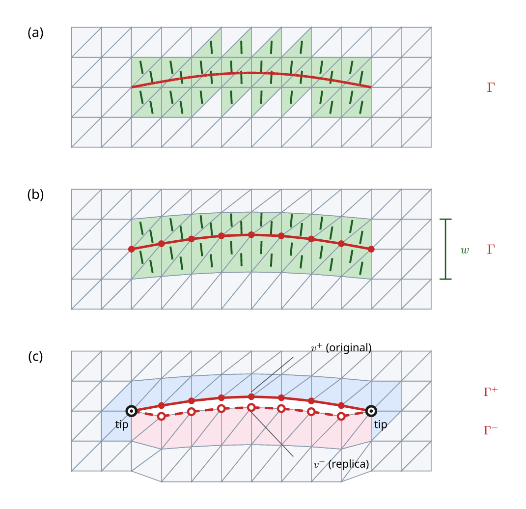
Figure 2:One fault, three strategies, on one mesh. (a) The non-conforming paint: the trace across the flat grid, and the band is whichever cells fall within of it. (b) The ribbon: the mesh is bent so that the same trace runs along element edges, and the band is the cells either side of it, each carrying a director; nothing is duplicated and every field is continuous. (c) The split, on the bent mesh: each interior vertex of the chain is duplicated and the cells on the Minus side are rewired to the replica; the tips are not duplicated. The copies are coincident — the lower block is pulled away only so that they can be seen.
Figure 2 compares the three strategies on one mesh. Panel (a) shows the fault running through the mesh with elements identified as fault / not-fault depending on their centroid distance to the fault. Panel (b) shows the ribbon near the fault constructed so that the fault volume itself is defined by element boundaries. Panel (c) is what the split does. The trace has first been made a chain of element edges, so that the two cells at every facet share it and every field is continuous across it, as anywhere else in the mesh. The split then duplicates each interior vertex of the chain. The original stays with the cells on one side, which we label Plus; the cells on the other side, Minus, are rewired to a replica at the same position. In this simple example, no elements are added or divided, but, across the fault, the two sides no longer share a degree of freedom, so the velocity is free to jump.
The fault is just the pair of surfaces and the condition we impose between each vertex and its replica. The simplest condition is no-opening: the two normal velocities of a pair are equal and the tangential velocities are free, which is a frictionless slippery interface. The slip rate is read off the pair as the tangential jump. A friction law is a relation between that jump and the traction the pair carries, and it lives on the pair as well.
The two end vertices of the chain are not duplicated. Slip therefore goes to zero at the tips, which is the crack condition, and the front of the fault needs no treatment of its own. This is also a limitation: a vertex that belonged to two chains would be a tip of each, pinned on both, so two cuts cannot meet.
Difficulties with branching faults
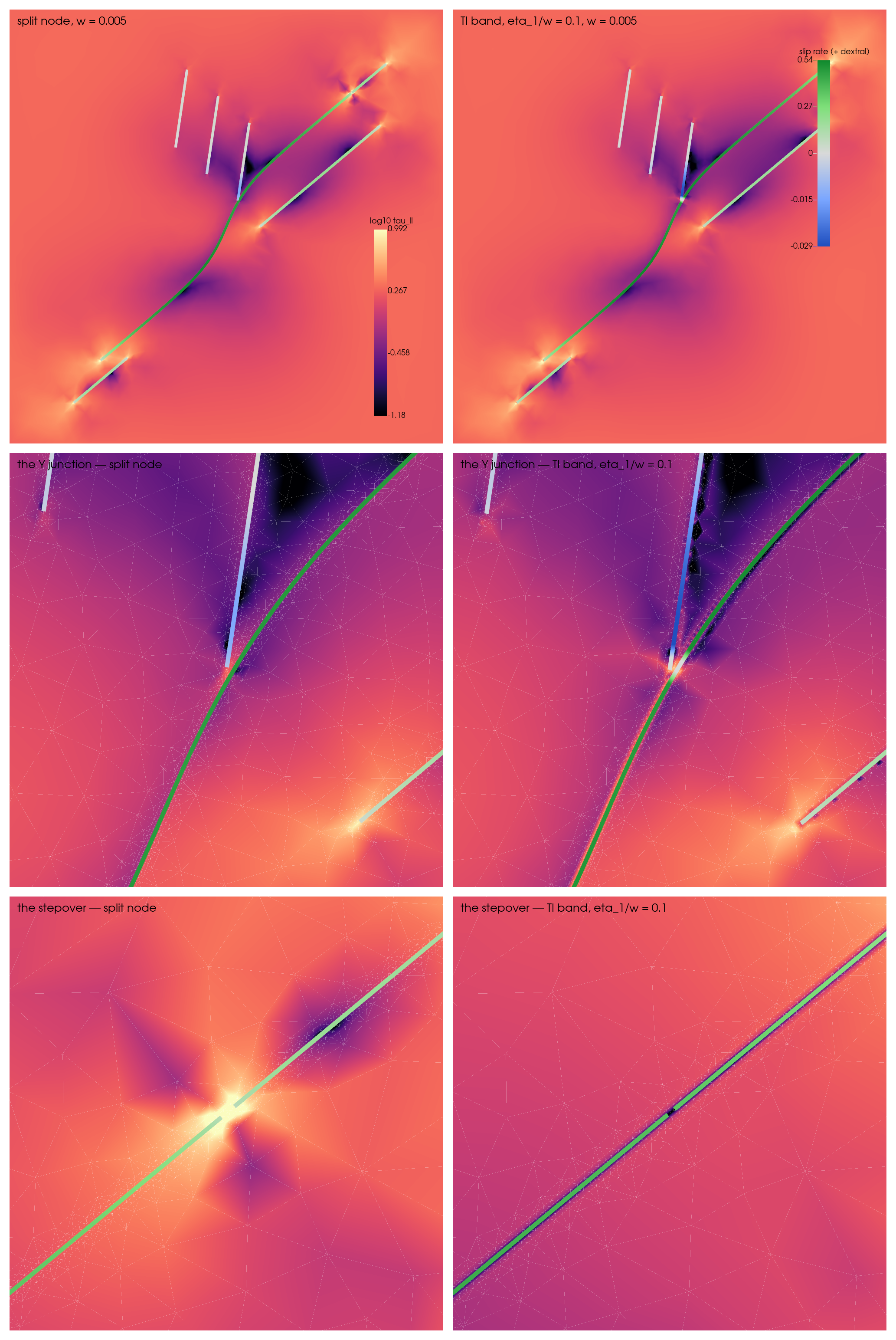
Figure 3:The same network as a cut (left) and as a band (right), both at with . Background: log10 of the second stress invariant on one scale. Traces: each representation’s own slip rate. Below, the Y junction, and the collinear stepover closed to one element — the least gap a cut can leave.
Consider one un-branched strand by itself. If we look at the slip rate across the fault for the transversely isotropic ribbon and compare it to the split mesh, we find that the two representations converge as the fault ribbon shrinks in width (in a background mesh of fixed resolution), provided the ratio remains fixed. The band’s mechanical strength is the ratio , not : halving the width at fixed viscosity effectively doubles the interface strength (see table).
| Main strand alone, peak slip rate | |||
|---|---|---|---|
| split | 0.5149 | 0.5154 | 0.5152 |
| TI band, | — | 0.5232 | 0.5133 |
| TI band, fixed | — | 0.5232 | 0.5000 |
Branching of the fault breaks this convergence because a junction is the one place where the two representations describe genuinely different objects. A band can fork: two weak zones meet and merge into one continuous weak region. Two cuts cannot: if they touch they would share a node that would carry two incompatible sets of constraints. The branch in the model is therefore represented slightly differently. The rheological bands merge smoothly in the mesh, but the cut branch stops short of the main fault.
The band’s junction is not free of choices either: in the cells the two bands share there can be only one director, and it is the orientation of whichever band was painted last.
Where the branches touch, slip is significantly higher, with a noticeable reversal of polarity in the slip orientation along the branch. The effect is present but more muted for the cut-in branch that does not quite reach the main fault.
The bottom row of Figure 3 is the same difficulty in its simplest form: two collinear segments of one fault, butted end to end with a single element between them. The cut has no choice about that element — two cuts that shared a vertex would pin it, so one element of intact rock is the least gap it can leave — and that ligament welds the two segments together. The segment beyond the gap carries two thirds of the slip a continuous fault carries there, the weld draws the main segment down by a few per cent as well, and refinement halves the weld’s length without ever removing it. The band has no such constraint: the two weak zones overlap and become one, the slip runs through unbroken, and the stress concentration at the buried tips disappears with it. Where a fault is segmented on the scale of the mesh rather than the scale of the model, this is the case for the band.
Choices
The split-node approach is by far the most efficient representation of a discontinuous, frictional fault that works well when the fault-width is completely unreachable with meshing. It does require cutting into the mesh each time the mesh is adapted or the fault is moved. The surface conditions are well-behaved when the solver sees them.
The transversely isotropic, meshed ribbon does a good job of faults that have branching structures or multiple, overlapping segments (or even segments that butt against each other). It requires mesh adaptation to keep the solver happy, and there is some tuning required to ensure the implementation converges to the split-node formulation.
The non-conforming transversely isotropic fault representation trades fault fidelity and solver efficiency against simplicity. This is the choice for cases where remeshing or mesh adaptation is difficult, and fluctuations in the near-fault stress-field can be tolerated.
- Davies, G. F. (1988). Role of the lithosphere in mantle convection. Journal of Geophysical Research: Solid Earth, 93(B9), 10451–10466. 10.1029/JB093iB09p10451
- Zhong, S., & Gurnis, M. (1995). Mantle Convection with Plates and Mobile, Faulted Plate Margins. Science, 267(5199), 838–843. 10.1126/science.267.5199.838
- Sandiford, D., & Moresi, L. (2019). Improving subduction interface implementation in dynamic numerical models. Solid Earth, 10(3), 969–985. 10.5194/se-10-969-2019
- Yang, H., Moresi, L. N., & Mansour, J. (2021). Stress recovery for the particle-in-cell finite element method. Physics of the Earth and Planetary Interiors, 311, 106637. 10.1016/j.pepi.2020.106637
- Sharples, W., Moresi, L.-N., Jadamec, M. A., & Revote, J. (2015). Styles of rifting and fault spacing in numerical models of crustal extension. Journal of Geophysical Research: Solid Earth, 120(6), 4379–4404. 10.1002/2014JB011813
- Moresi, L., & Mühlhaus, H.-B. (2006). Anisotropic viscous models of large-deformation Mohr–Coulomb failure. Philosophical Magazine, 86(21–22), 3287–3305. 10.1080/14786430500255419