How Underworld3 Turns SymPy into C

In a previous post we described why Underworld3 uses SymPy as its expression language and what that choice made possible. Here we'll go one level deeper: what actually happens between the moment you write a mathematical expression in Python and the moment PETSc receives a finite element term in the form of compiled C? The answer is a pipeline with six stages, and understanding it explains most of what makes UW3 tick.

At the User Level

A typical Underworld3 setup might look like this:

import underworld3 as uw
import sympy

# Parameters as UWexpressions — symbolic names with concrete values and units
eta_0   = uw.expression("eta_0", uw.quantity(1e21, "Pa*s"))    # reference viscosity
gamma   = uw.expression("gamma", 13.8)                         # FK sensitivity (dimensionless)
rho     = uw.expression("rho", uw.quantity(3300, "kg/m**3"))   # density
gravity = uw.expression("g", uw.quantity(9.8, "m/s**2"))       # gravitational acceleration

# Temperature is a mesh variable — a field solved on the mesh
T = uw.discretisation.MeshVariable("T", mesh, 1, degree=2)

# Frank-Kamenetskii viscosity: η = η₀ exp(-γ T)
# This is a SymPy expression built from UWexpressions and a MeshVariable
viscosity_fn = eta_0 * sympy.exp(-gamma * T)

# Set up the Stokes solver
stokes = uw.systems.Stokes(mesh)
stokes.constitutive_model = uw.constitutive_models.ViscousFlowModel
stokes.constitutive_model.Parameters.shear_viscosity_0 = viscosity_fn
stokes.bodyforce = -rho * gravity
stokes.solve()

The viscosity here is a SymPy expression. eta_0 and gamma are UWexpressions (symbols that carry values), T is a mesh variable (a symbol that represents spatial field data), and sympy.exp is ordinary SymPy. The solver does not care what the expression contains — constant, field-dependent, nonlinear — it handles them all the same way. What happens behind solve() is the subject of this post.

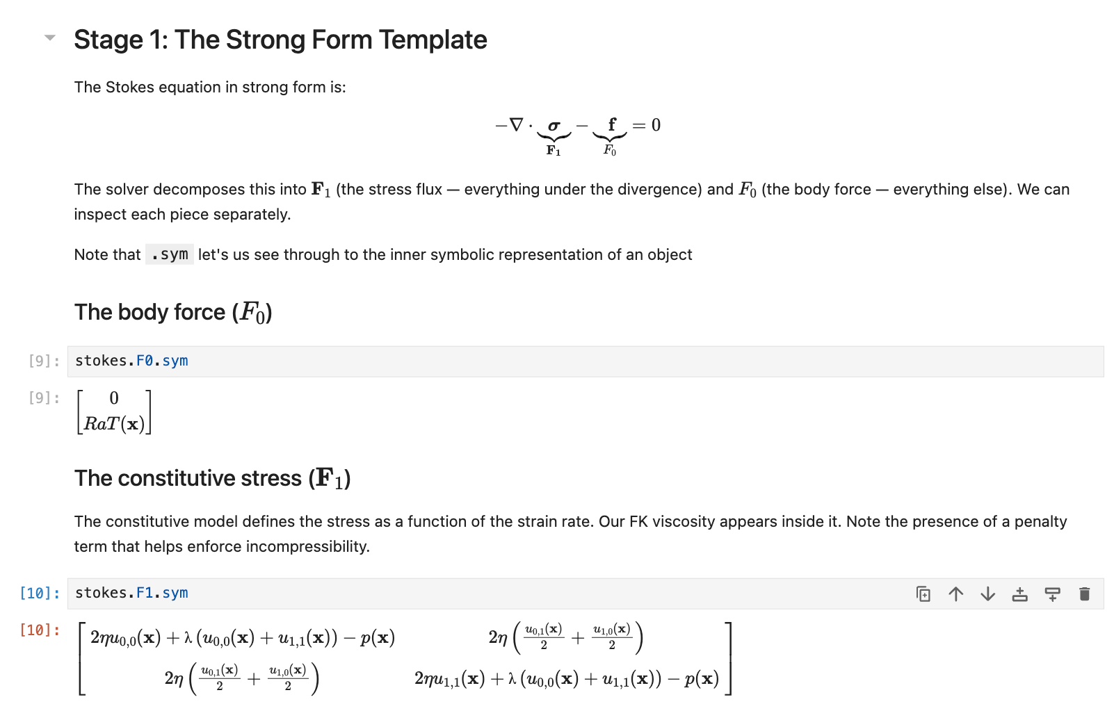
Stage 1: The Strong Form Template

Every UW3 solver defines a strong-form PDE template. For Stokes flow, this is:

$$ -\nabla \cdot \underbrace{\boldsymbol{\sigma}(u, \nabla u)}_{\mathbf{F_1}} - \underbrace{\mathbf{f}(u, \nabla u)}_{F_0} = 0
$$

The solver decomposes this into two symbolic properties: $\mathbf{F_1}$ (flux-like terms: everything under a divergence operator, which is then paired with gradients of the test function in the weak form) and ${F_0}$ (force-like terms: everything else). For Stokes, $\mathbf{F_1}$ contains the constitutive stress minus the pressure, while ${F_0}$ contains the body force and any time-derivative contributions.

These are ordinary SymPy expressions. You can inspect them and they render beautifully in a notebook.

The solver does not evaluate these expressions. It stores them symbolically and defers everything until the moment they are converted (compiled) into C functions.

Stage 2: Automatic Jacobians

PETSc's Newton solver (SNES) needs not just the residual but its derivative with respect to the unknowns. In many finite element codes, someone has to derive these by hand and code them in C. In UW3, SymPy does it. We did not use PETSc Newton solvers in Underworld2 because we had no systematic way to produce Jacobians for arbitrary user-defined constitutive models contructed from python functions.

The solver takes $F_0$ and $F_1$ and differentiates them with respect to the unknown field and its gradient, producing four Jacobian blocks:

 $G_0 = ∂F_0/∂u$       $G_1 = ∂F_0/∂(∇u)$
 $G_2 = ∂F_1/∂u$       $G_3 = ∂F_1/∂(∇u)$

This is sympy.derive_by_array() applied to the user's constitutive law. For a simple linear viscosity, $G_3$ is just the viscosity tensor. For a nonlinear rheology (strain-rate-dependent, pressure-dependent, with yield criteria) the derivatives can be complex, and SymPy computes them exactly. No finite-difference approximations, no hand-coding. What is more, they can be checked through introspection and interaction because they are symbolic before and after differentiation.

The Symbolic Wrappers

Before we describe how expressions are compiled, it helps to understand how they are constructed. UW3 does not use plain SymPy symbols. It wraps them in objects that carry extra information — and the reason is lazy evaluation.

UWexpression. A SymPy Symbol that holds a value inside it. When you write eta = uw.expression("eta", 1e21), you get a symbol that behaves like any SymPy variable in an expression tree — you can multiply it, differentiate through it, simplify around it — but it also knows that its current value is $10^{21}$. The expression tree stays symbolic for as long as you want to inspect or manipulate it. When the JIT compiler finally needs a number, it reaches inside the wrapper and extracts the value.

Why not use a plain SymPy symbol? Because a plain symbol eta is purely abstract — it has no value. And a plain number 1e21 cannot participate in symbolic differentiation. UWexpression bridges the gap: symbolic identity for the algebra, concrete value for the compiler. What's more, differentiation is lazy: we can differentiate an expression and, if we change sub-expressions or their values, the result will be computed correctly at the time we use the derivative.

MeshVariable symbols. When you create a mesh variable for velocity or temperature, it acquires a .sym property — a SymPy Matrix of special symbols that represent the field. These symbols know they are spatial data living on the mesh, not parameters. At compile time, they get patched to C array accessors: the velocity unknown becomes petsc_u[0], an auxiliary temperature field becomes petsc_a[3].

Spatial gradients of mesh variables are also symbols. When you write T.diff(x), UW3 intercepts the call and returns a dedicated gradient symbol — it does not try to evaluate the derivative. This symbol represents $\partial T / \partial x$ abstractly, and at compile time it gets patched to petsc_u_x[0] or petsc_a_x[0]. PETSc provides the numerical gradient value at each quadrature point during assembly.

This means the two kinds of derivative in UW3 work together naturally. The automatic Jacobian derivation (Stage 2) uses SymPy's chain rule to differentiate through gradient symbols: if the stress depends on $\nabla u$, and the Jacobian needs $\partial \mathbf{F}_1 / \partial (\nabla u)$, SymPy applies the chain rule symbolically, and the gradient symbols survive into the generated C as array references. No derivative is ever evaluated numerically until PETSc runs the compiled callback at a quadrature point.

Coordinates. The mesh coordinates themselves are SymPy symbols. mesh.X[0] is $x$, mesh.X[1] is $y$. You use them in expressions naturally — rho * g * mesh.X[1] for a depth-dependent body force — and at compile time they become petsc_x[0], petsc_x[1]. In spherical coordinates, the same mechanism provides $r$, $\theta$, $\phi$ with the correct differential geometry, and sympy.diff(f, x) gives $df/dx$ in whatever coordinate system the mesh uses.

UWQuantity. An expression that carries physical units (via Pint). If the user specifies eta = uw.quantity(1e21, "Pa*s"), the units track through all arithmetic. At compile time, quantities are non-dimensionalised — the solver always works in scaled, dimensionless space. The units exist for the user's benefit: display, validation, dimensional analysis. PETSc never sees them.

The point of all these wrappers is that the expression tree the user builds is simultaneously human-readable mathematics (inspect it, render it in a notebook, check the units) and a complete specification for C code generation. Nothing is lost between the two views.

Stage 3: Unwrapping

With that context, the next step is easy to follow. The expressions coming out of Stage 2 are full of these user-facing wrappers. Before generating C code, the compiler must resolve them to pure SymPy — extracting values, stripping units, mapping field symbols to array indices.

Everything that reaches PETSc must be dimensionless. If we want to work with physical units — viscosity in Pa·s, density in kg/m³ — the unwrapping stage needs to non-dimensionalises all values using the reference quantities that we define at the start of the computation. This applies to constants and field data alike. PETSc never sees a unit; it works in scaled, dimensionless space throughout.

The unwrapping happens in two phases.

Phase 1: Extract constants. The compiler scans the expression tree for UWexpressions that have no spatial or field dependencies — things like viscosity parameters, time-step size, penalty coefficients. These are pulled out, non-dimensionalised, and assigned indices in a flat array. In the generated C code, they appear as constants[0], constants[1], and so on. Their current (dimensionless) values are passed to PETSc at solve time, not baked into the compiled code.

This is important. If you change (for example) a viscosity parameter between solves, UW3 does not recompile anything. It re-packs the constants array with the new dimensionless value and PETSc picks it up on the next assembly pass.

Phase 2: Resolve everything else. The remaining UWexpressions — field variables, coordinates, compound expressions — are recursively unwrapped to their underlying SymPy forms. Coordinate symbols are resolved to their SymPy BaseScalar representations. Any remaining UWQuantities are non-dimensionalised.

The result is a set of pure SymPy expressions with two kinds of atoms: constants (indexed placeholders) and field variables (which will be patched to C array references in the next stage).

Stage 4: C Code Generation

Now the compiler turns SymPy into C. Each mesh variable in the expression — the unknown field, its gradient, auxiliary fields like temperature or pressure — gets patched with a C accessor string. The unknown field u becomes petsc_u[0]; its x-gradient becomes petsc_u_x[0]; an auxiliary mesh variable becomes petsc_a[offset]. Coordinate variables become petsc_x[0], petsc_x[1], petsc_x[2].

SymPy's C99 code printer then converts the patched expression to a C string. The compiler wraps this in a function with the exact signature that PETSc's DMPlex assembly expects:

void fn_residual_F1(
     PetscInt dim, PetscInt Nf, PetscInt NfAux,
     const PetscInt uOff[], const PetscInt uOff_x[],
     const PetscScalar petsc_u[],       // unknown field values
     const PetscScalar petsc_u_x[],     // unknown field gradients
     const PetscInt aOff[], const PetscInt aOff_x[],
     const PetscScalar petsc_a[],       // auxiliary fields
     const PetscScalar petsc_a_x[],     // auxiliary field gradients
     PetscReal petsc_t,                 // time
     const PetscReal petsc_x[],         // coordinates
     PetscInt numConstants,
     const PetscScalar constants[],     // runtime parameters
     PetscScalar out[]                  // output
 ) {
     out[0] = constants[0] * petsc_u_x[0] + ...;
 }
 

A linear viscous Stokes problem generates a handful of simple functions. A nonlinear rheology with pressure-dependent yielding generates longer ones, but the process is identical: SymPy handles the complexity.

Stage 5: Compilation and Loading

The generated C code, a Cython wrapper, and a build script are written to a temporary directory. A subprocess call to python setup.py build_ext --inplace compiles everything to a shared library. The library is loaded via Python's import machinery, and function pointers are extracted.

Compilation can be expensive, a second or more per function, so UW3 caches aggressively. The cache operates at the level of individual functions, not entire solvers. Each of the $F_0$, $F_1$, $G_0$–$G_3$ residual and Jacobian callbacks is hashed independently based on its structural form: the expression with constants replaced by placeholders. Two consequences follow.

First, changing a parameter value (viscosity, density, time-step size) does not trigger recompilation. The structural form has not changed — only the values in the constants array, which are updated cheaply at solve time.

Second, functions that are shared between solvers are compiled once. If a Stokes solver and an advection-diffusion solver both reference the same temperature field with the same constitutive expression, the cached compiled function is reused. In a coupled multiphysics problem with several solvers, this avoids a great deal of redundant compilation.

Each JIT module gets a random symbol prefix to avoid name clashes when multiple compiled libraries coexist in the same process.

Stage 6: PETSc Takes Over

The function pointers are registered with PETSc's DMPlex via PetscDSSetResidual() and PetscDSSetJacobian(). From this point, PETSc owns the assembly. During each Newton iteration, PETSc loops over mesh elements, evaluates the compiled functions at quadrature points, and assembles the global residual and Jacobian matrices.

Before each solve, UW3 packs the current values of all constants and passes them to PETSc via PetscDSSetConstants(). This is how time-varying parameters, continuation parameters, and BDF/Adams-Moulton coefficients reach the compiled C code without recompilation.

The user calls solver.solve(). PETSc runs Newton iterations, calling back into the JIT-compiled functions thousands or millions of times. The SymPy expressions that the user wrote in a notebook are now running as native C inside PETSc's optimised assembly loops.

The Complete Chain

To summarise the pipeline for a single constitutive model:

1. User writes SymPy expressions for stress, body force, boundary conditions
2. Solver derives Jacobian blocks automatically via symbolic differentiation
3. Compiler extracts runtime constants (parameters that can change between solves)
4. Compiler unwraps remaining expressions to pure SymPy, patches field variables to C accessors
5. SymPy prints the expressions as C99 code inside PETSc-compatible function signatures
6. Subprocess compiles to a shared library, which is cached and loaded
7. PETSc registers the function pointers and uses them during finite element assembly
8. At each solve, current constant values are packed and passed to PETSc

The entire chain is transparent. At any stage, you can inspect what the code has done: view the symbolic expression, view the generated C, view the Jacobian that SymPy derived. In a Jupyter notebook, the solver will render the mathematics it assembled. This is what we mean when we say UW3 is self-describing.

Why This Design

Other finite element frameworks take a different approach. FEniCS and Firedrake use the Unified Form Language (UFL) to describe the weak form directly. The user writes the variational problem; the framework compiles it. This is elegant and powerful, but the user works with the weak form themselves which, for many people, is a non-trivial step, especially for complex constitutive models with multiple coupled fields.

UW3 starts from the strong form — the same form that appears in textbooks and publications. The framework handles the weak-form transformation, the Jacobian derivation, and the code generation. The cost is that we rely on PETSc's pointwise function template, which constrains the weak form to a specific decomposition. The benefit is that domain scientists work at the level of equations, not variational calculus.

For geodynamics, where constitutive models are complex, nonlinear, and frequently changed during model development, this trade-off has worked well. The barrier to trying a new rheology is writing a Python class, not deriving a weak form and coding its Jacobian in C.

The Underworld project is supported by AuScope and the Australian Government through the National Collaborative Research Infrastructure Strategy (NCRIS). Source code: github.com/underworldcode/underworld3