Compressible convection in cartesian coordinates with Underworld3

Introduction and benchmarking

The convection of the Earth’s mantle is usually modelled as an incompressible process, referred to as the Boussinesq approximation. However, in the Earth’s mantle, the pressure increase associated with depth also increases the density due to self-compression (King et al. 2010). In some applications, this compressibility may be non-negligible and modelling it may be desirable. Over the years, several mantle convection formulations have been devised to take this compressibility into account. One such formulation is the Truncated Anelastic Liquid Approximation (TALA) (Ita and King, 1994; Jarvis and Mckenzie, 1980). In this approximation, a depth-depended reference profile is defined which dictates how the density varies with depth. This is subsequently used to calculate the volumetric changes as a result of pressurization and heating (Gassmöller et al., 2020). In addition, the buoyancy term in the momentum equation precludes the contributions of the density changes due to pressure variations (van Zelst et al., 2022). Taking compressibility into account adds temperature gradients and adiabatic density which increases the complexity of mantle dynamics (Tan and Gurnis, 2007). Here, we easily implement an isoviscous compressible convection model with the Truncated Anelastic Liquid Approximation (TALA) formulation in cartesian coordinates using Underworld3.

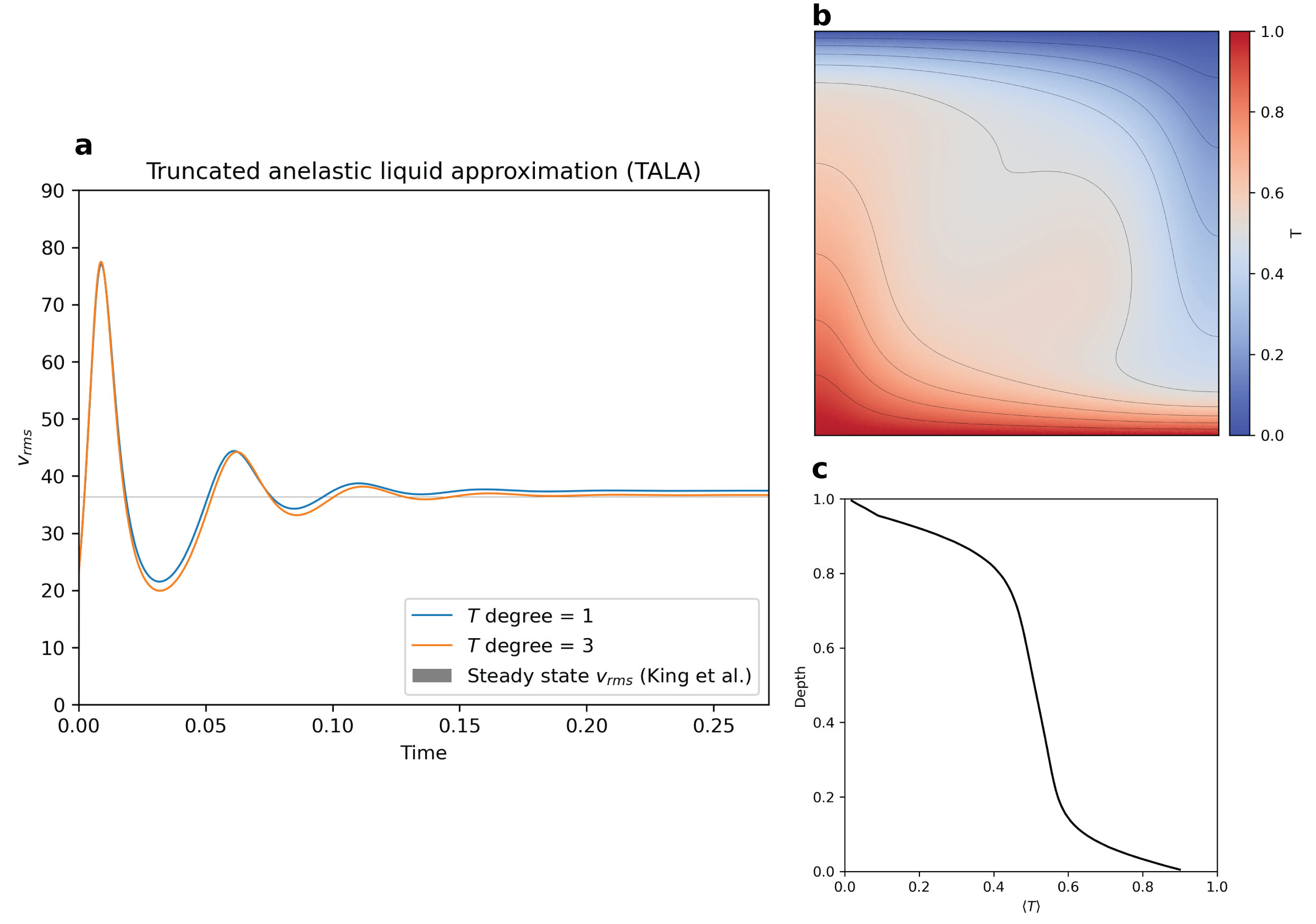
To benchmark the implementation of TALA in Underworld3, we compare the measured steady-state root mean squared velocity, $v_{rms}$, to the values reported in (King et al., 2010). The compressible convection implementation in Underworld3 reaches a steady-state, as shown in the $v_{rms}$ as a function of time plot in Figure 1a. We’ve also tested how close the steady-state $v_{rms}$ is to those reported in (King et al., 2010). Using a temperature polynomial degree of 1 gets us close to the reported range with a relative difference of ~3%. Increasing the polynomial degree to 3 further reduces the relative difference to less than 1%, as shown in Figure 1a. We also show the temperature field when steady-state is reached in Figure 1b and the laterally-averaged temperature as a function of depth in figure 1c.

The implementation codes together with the steady-state temperature, pressure, and velocity fields are found in https://github.com/underworld-community/UW3-benchmarks/blob/dev/Working/Cartesian/Ex_Convection_TALA_benchmark.py.

After this, we aim to benchmark the TALA implementation against other test cases and to implement the slightly more complicated Anelastic Liquid Approximation (ALA) formulation. We're also targeting to implement compressible convection in an annulus configuration. Stay tuned!

Important implementation details

If I still have your attention at this point, why not continue and check out how we did this? For the important implementation details, read ahead! =)

In compressible convection, the total temperature, $T$, pressure, $P$, and density, $\rho$, are expressed as a sum of a reference state (overbarred) and a perturbation (primed). That is:

$$ T = \bar T + T' ; \space \space \space p = \bar p + p' ; \space \space \space \rho = \bar \rho (\bar T, \bar p) + \rho' \space \space \space (1) $$

Assuming an adiabatic Adams-Williamson equation of state (Birch, 1952; King et al., 2010), and non-dimensionalising the equations, the reference states are expressed as:

$$ \bar \rho = \rho_{o} \exp \left( \frac{\textrm{Di}} {\gamma_R} \left( 1 - z \right)\right); \space \space \space
\bar T = T_s \left( \exp\left(\textrm{Di} (1-z) \right) - 1\right) \space \space \space (2)$$

Where $ \rho_o$ is a non-dimensionalised surface density, Di is the dissipation number, $\gamma_R$ is the Grüneisen parameter, $T_s$ is the non-dimensionalised surface temperature, and $z$ is the non-dimensionalised depth.

Setting-up the Stokes' equations

Underworld, a particle-in-cell finite element modelling code, is now in its third major iteration. With the upcoming version, implementing compressible convection has never been easier. To do so, we only need to modify the Stokes’ and Advection-Diffusion equations accordingly.

For compressible convection, the conservation of mass is expressed as:

$$ \nabla \cdot (\bar \rho \vec u) = \nabla \cdot \vec u + \frac{1}{\bar \rho} \vec u \nabla \bar \rho = 0. \space \space \space (3)$$

The conservation of momentum is given as

$$\nabla \cdot [\eta (\nabla \vec u + \nabla \vec u^T - \frac {2}{3}\nabla \cdot \vec u \mathbf{I})] - \nabla p' - \textrm{Ra} \bar \rho \bar g \bar \alpha (T - \bar T)= 0, \space \space \space (4)$$

while the deviatoric strain tensor, $\tau$, is

$$\tau = 2 \eta \dot \epsilon = \eta (\nabla \vec u + \nabla \vec u^T - \frac {2}{3}\nabla \cdot \vec u \mathbf{I}). \space \space \space (5)$$

In these equations, $\vec u$, $p'$, $T$ and $\dot \epsilon $ are the velocity, pressure, total temperature, and strain rate, respectively. In addition, $\bar g$, $\bar \alpha$, $\eta$, and Ra are the gravity, expansivity, viscosity, and Rayleigh number, respectively.

Key to the ease of implementing compressible equation is the use of Sympy in Underworld3 to symbolically define additional terms into the default systems of equations. We first define the depth-dependent reference values of density and temperature as:

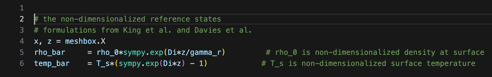
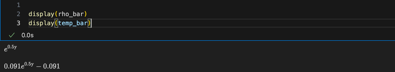
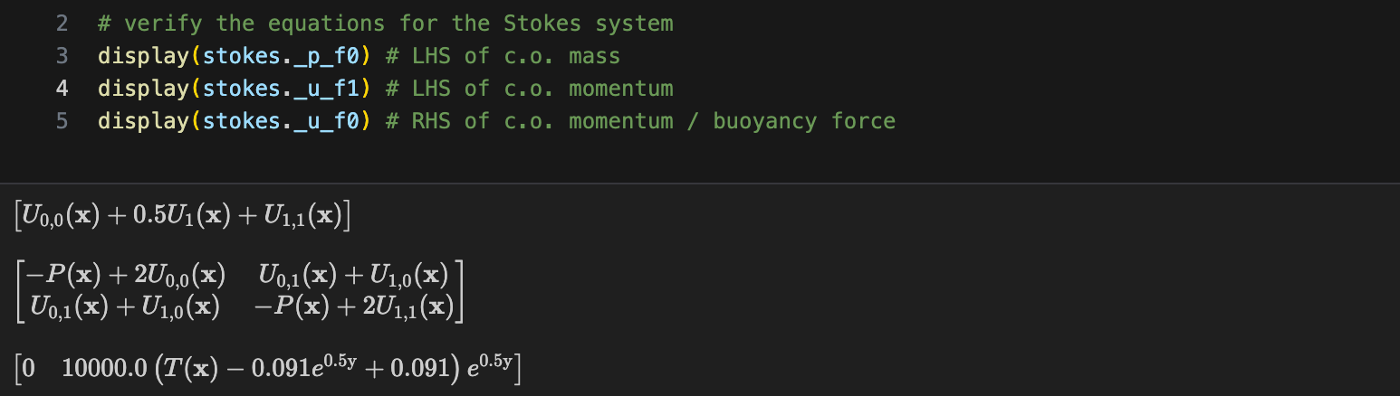
The first line stipulates that we wish to assign the symbolic representations of the meshbox coordinates to variables. The next ones indicate that we are expressing the reference functions as Sympy expressions. We can use the display() function to check what these symbolically look like:

Next, we add the necessary terms into the Stokes equations (see Equations 3 and 4). This is done in the following lines of code, assuming that the usual methods to set-up a Stokes solver object have been done:

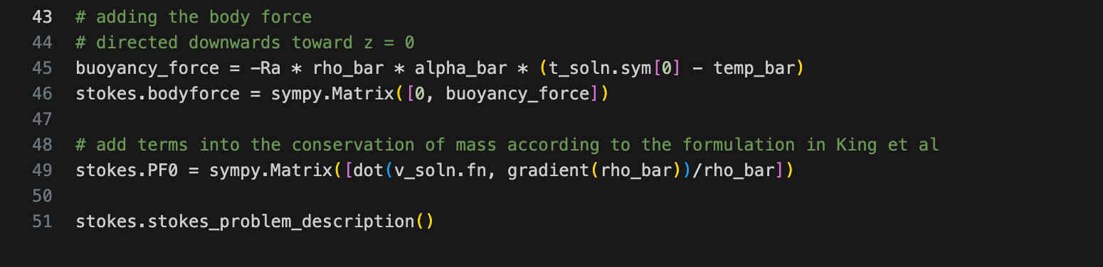
The first two lines of code is for setting up the body force in both the x- and z- coordinates. The third line adds the velocity divergence term in the momentum conservation equation, while the fourth line is for adding the effect of a depth-dependent density in the conservation of mass. Note that all of these are defined symbolically. Again, using the display function to check the changes done, we get:

Next, we set-up the Advection-Diffusion system. For the TALA formulation, the conservation of energy in terms of the total temperature, $T$, is given as:

$$ \frac{DT}{Dt} - \frac{\textrm{Di} \bar \alpha}{\bar c_p}\vec g \cdot \vec u (T + T_s) = \frac {1} {\bar \rho \bar c_p} \nabla \cdot (\bar k \nabla T) + \frac{\textrm{Di}}{\textrm{Ra}} \frac{1}{\bar \rho \bar c_p} \phi \space \space \space (6)$$

Where $\bar c_p$ is the heat capacity, $\bar k$ is the diffusivity, and $\phi$ is the viscous dissipation (Davies et al.). The viscous dissipation is calculated using the expression:

$$ \phi = \frac{1}{2}\tau:\dot{\epsilon} \space \space \space (7)$$

To add the terms associated with adiabatic heating and viscous dissipation, we do the following:

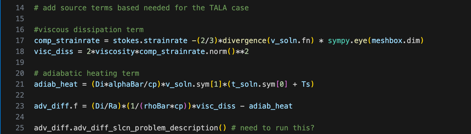
In the code snippet above, the first three lines are for symbolically defining the terms associated with the viscous dissipation and adiabatic heating (see Equations 4 and 5). The last one is for adding the two terms into the original advection-diffusion equation. Note the appropriate changes in sign as we move the terms to the right hand side of the equation and the convention we set for the direction of gravity.

The changes result to a model of isoviscous convection under the Truncated Anelastic Liquid Approximation (TALA). The rest of the code is very similar to how convection under the Boussinesq approximation is done. Have a look at the entire code and try it out yourself! Have fun learning!

References:

Birch, F., 1952. Elasticity and constitution of the Earth’s interior. Journal of Geophysical Research (1896-1977) 57, 227–286. https://doi.org/10.1029/JZ057i002p00227

Davies, D.R., Kramer, S.C., Wilson, C.R., Tosi, N., Besserer, J., Huttig, C., n.d. A community benchmark for compressible mantle convection in a two–dimensional cylindrical domain.

Gassmöller, R., Dannberg, J., Bangerth, W., Heister, T., Myhill, R., 2020. On formulations of compressible mantle convection. Geophysical Journal International 221, 1264–1280. https://doi.org/10.1093/gji/ggaa078
Ita, J., King, S.D., 1994. Sensitivity of convection with an endothermic phase change to the form of governing equations, initial conditions, boundary conditions, and equation of state. Journal of Geophysical Research: Solid Earth 99, 15919–15938. https://doi.org/10.1029/94JB00852
Jarvis, G.T., Mckenzie, D.P., 1980. Convection in a compressible fluid with infinite Prandtl number. Journal of Fluid Mechanics 96, 515–583. https://doi.org/10.1017/S002211208000225X
King, S.D., Lee, C., van Keken, P.E., Leng, W., Zhong, S., Tan, E., Tosi, N., Kameyama, M.C., 2010. A community benchmark for 2-D Cartesian compressible convection in the Earth’s mantle. Geophysical Journal International 180, 73–87. https://doi.org/10.1111/j.1365-246X.2009.04413.x
Tan, E., Gurnis, M., 2007. Compressible thermochemical convection and application to lower mantle structures. Journal of Geophysical Research: Solid Earth 112. https://doi.org/10.1029/2006JB004505
van Zelst, I., Crameri, F., Pusok, A.E., Glerum, A., Dannberg, J., Thieulot, C., 2022. 101 geodynamic modelling: how to design, interpret, and communicate numerical studies of the solid Earth. Solid Earth 13, 583–637. https://doi.org/10.5194/se-13-583-2022