
A geodynamic model with a uniform mesh, almost certainly expends most of its resolution in the wrong places. The features that need small cells: a thermal boundary layer; a shear band; a subducting slab’s megathrust zone, each occupy a few percent of the domain and usually move around during the calculation. Mesh refinement is important, and so is the ability to respond to changes in where the refinement is needed.
When the requirements for refinement change throughout the computation, we have to undertake an adaptive mesh refinement each step, or every few steps. Conceptually, the simplest way to do this is to build a new mesh with exactly the resolution we need, then transfer all the problem data to the new mesh. This will give us the ideal mesh for the problem, but it does mean navigating and interpolating between meshes and is particularly tricky in parallel.
An alternative is to add resolution to the mesh where and when it is needed, starting from a base mesh which we keep as a reference point for the duration of the calculation. Much of the mesh then remains unchanged and we only need to move data in areas where nodes have been added. Because we are limited to splitting existing elements, however, there are some limits to how “nice” a mesh we can construct.
An alternative to these form of refinement is to deform the grid so the nodes bunch up where additional resolution is required and become more widely spaced elsewhere. A fixed node budget, deployed as effectively as possible while maintaining mesh quality.
We’ll show how mesh-redisribution can be done, what sort of resolution improvements we can achieve, and discuss the advantages / disadvantages of this way of doing things. But first, some background.
What refinement charges
Refinement changes the points in the mesh, and in a parallel run three things follow.
The partition may no longer be balanced. New cells appear where the physics is interesting, which is to say unevenly, so the ranks that own the interesting region end up owning most of the work. Fixing that means repartitioning and migrating — cells, degrees of freedom, every field, and any particles riding along. That migration is not a detail of the implementation. It is communication proportional to how much the mesh changed, and it happens every time the mesh changes.
Fields have to be transferred between meshes that share no nodes. The old and new meshes are related by the refinement rule, but the values live at places that do not correspond, and interpolating between them costs accuracy every time. Do it every ten steps for a thousand steps and the transfer error is a term in your answer.
The multigrid hierarchy must be re-derived. Remeshing or refining the existing mesh means creating a new hierarchical relationship between nodes on the nesting of the grids.
Distort the mesh, don’t re-mesh
There is an alternative to re-meshing that does not require repartitioning or recontructing the hierarchical nature of the grid. It may not require remapping the data under some circumstances. We stretch the grid, like an elastic net, allowing the points to move but to stay connected to their neighbours.
When the node budget is fixed, no node is created, none is destroyed, and no cell changes its neighbours. Every node stays on the rank that owned it. What moves is where the nodes are — they slide to where the resolution is wanted and away from where it is not.
Much of what makes refinement complex and expensive is then absent by construction:
the partition is unchanged, because ownership is a property of the point set and the point set did not change;
the connectivity is unchanged, so the multigrid hierarchy — which is built from the topology, not from the coordinates — is still a hierarchy;
there is no mesh-to-mesh transfer, because there is only one mesh.
What you give up is equally clear, and we will come back to that: a fixed budget of nodes can only be redistributed, never increased.
Equidistribution is not mesh optimisation
As with any simple idea, the practical implementation is often full of traps. Redistributing a mesh is a global operation: nodes all need to move in synchrony and they cannot overtake each other or the mesh becomes tangled an unusable. These are constraints that ultimately limit how much we can improve mesh resolution.
The algorithm that we need is equidistribution: supply a metric — a monitor function saying how much resolution is wanted, and in a tensor metric, in which direction — and ask for the map from a fixed computational mesh to the physical mesh under which every cell carries the same amount of . That is a Monge–Ampère-style problem, and it is the same target the refiner is chasing; the difference is only that the refiner is allowed to add nodes and we are not.
Underworld3 solves it with the Huang–Kamenski moving mesh PDE 1, which generates the physical mesh as the image of a fixed computational mesh under the inverse coordinate map, minimising
with , the Jacobian of the map between the reference and physical elements, and . The first term is the shape term, the second the size term.
Two properties of that functional are why this is the mover we use and not one of the several we retired.
It cannot fold the mesh. as , so a cell cannot be driven through zero volume without the energy going to infinity first. That is a theorem about the functional 2, not a guard bolted on afterwards, and it is the difference between a mover you can leave running in a time loop and one you have to watch.
It aligns as well as clusters. is a tensor, so a metric that is thin across a fault normal and long along it produces cells that are thin across the fault and long along it. An isotropic monitor function can only ask for smaller cells; a tensor one can ask for the right cells, which for a sheet-like feature is worth far more than the same node count spent isotropically.
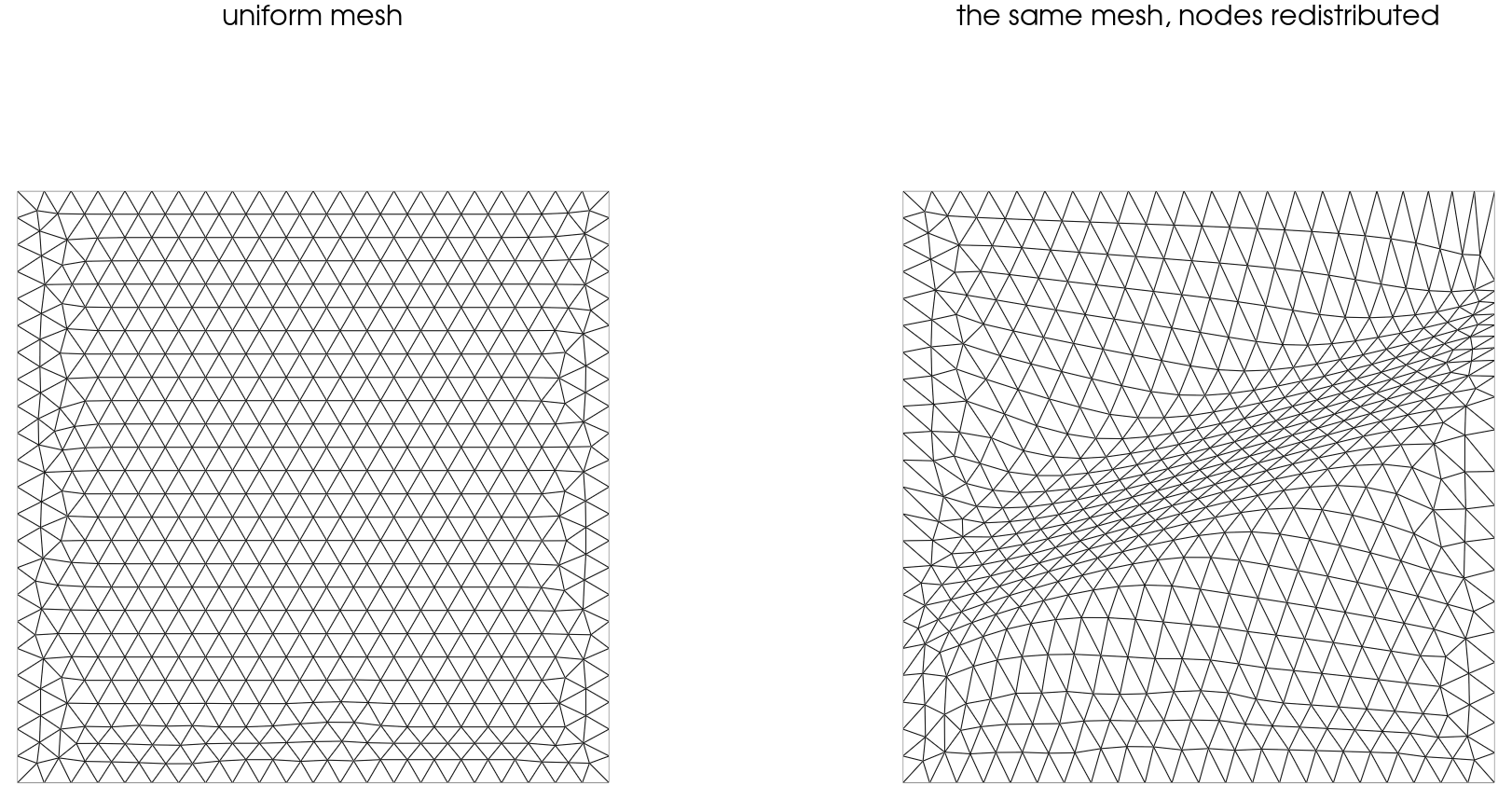
The same mesh, before and after redistribution to an anisotropic metric across a diagonal band. Both panels have 1152 cells and 621 nodes — the counts are not merely similar, they are the same mesh object at two moments. What changed is where the nodes are: the median cell on the band is 1.65× smaller than in the bulk, and the cells there are visibly stretched along the band rather than simply shrunk. Nothing was refined, nothing was transferred between meshes, and no node changed rank.
In use it is two calls:
import underworld3 as uw

# A scalar metric from |grad T|. refinement=R asks for cells up to R
# times finer than the BACKGROUND spacing h0, not a finest:coarsest
# ratio: with coarsening="auto" the sparsest cells relax to h0*R**(1/d),
# so the full envelope is [h0/R, h0*R**(1/d)].
rho = uw.meshing.metric_density_from_gradient(
    mesh, T, refinement=5, coarsening="auto",
    metric_choice="front-following")

# Move the nodes. The mover owns field transfer: it remaps T, carries
# the semi-Lagrangian history and fires the on_remesh hooks.
uw.meshing.node_redistribution(
    mesh, rho,
    method_kwargs=dict(step_frac=0.2, accel="none", momentum=0.0,
                       n_outer=400),
    slip_surfaces=True,      # boundary nodes slide tangentially
    skip_threshold=0.9)      # don't move an already-aligned mesh
accel selects how the outer iteration is driven. The unaccelerated descent
above is the setting to reach for when the grading you get is weaker than the
grading you asked for; it needs more outer iterations and it converges
reliably. We come back below to telling a mover that has finished from one
that has stalled.
Data updates are still needed
It would be nice to say no field transfer is needed but it’s not true. Nodes move, so the value stored at a node is now the value of the old field at a place the node used to be, and it has to be re-evaluated. That is an interpolation and it costs us in accuracy once we evaluate the update.
What it does not cost is communication. A node moves a fraction of a cell diameter, so the point it must be evaluated at lies in its own patch or one owned by a neighbour — inside the halo the mesh already maintains. Compare the full remeshing case, where source and target are unrelated meshes and locating a point can land anywhere in the domain, on any rank, requiring a parallel search and then a migration to answer it. Same operation in name; entirely different in cost and in who has to talk to whom.
Setting a reference frame
The functional measures a cell’s distortion against a reference element. By default, the reference is the mesh as it was on the first call. That is the correct choice for redistribution — we are asking for a map from this mesh to a better-graded one — and it has a consequence that is quite easy to miss.
Under a uniform metric, a distorted mesh is its own optimum. If
then in every cell, the shape
gradient is zero everywhere, and the mover does nothing. Not approximately, exactly.
The measured displacement of redistribute_nodes under
is exactly zero. Handed a mesh full of needle-shaped elements,
for example, the redistributor does not drive towards a more evenly distributed
mesh as, intuitively, we might at first expect.
But, if we replace each cell’s reference element with a single regular simplex, scaled to that cell’s own current volume, the same functional describes the distortion “away from equilateral” rather than “away from the mesh I was handed”. Because each reference is scaled to the cell’s own volume, at entry, so the size term starts at its optimum and stays there — the grading is preserved and only shape does work.
Three frames, then, from one piece of machinery:
reference | the reference element is | what it does |
|---|---|---|
"mesh" | the mesh at first call | redistribute to a metric |
"ideal" | a regular simplex at each cell’s own volume | repair shape, hold size |
"ideal-metric" | a regular simplex at one common volume | repair shape, metric sets size |
The user-facing call is mesh.relax() for the metric-free case and
mesh.relax(M) for the third, alongside mesh.redistribute_nodes(M) for the
first.
The ceiling is set by the node budget
A mover redistributes; it never adds a node. Starting from a uniform mesh it saturates — about 1.8× finer on a fault than in the background — and no amount of iteration goes past that. The nodes it would need are somewhere else, and if the metric has ridges between where the nodes are and where we want them, the algorithm cannot push nodes over that barrier.
We can see this limit directly if we add in the nodes that the redistribution needs when we initially mesh the domain. If we put a refinement into the base mesh, the mover does not merely maintain it, it compounds it. In the table below, we try to resolve a (linear) fault zone. If we pre-refine the mesh with gmsh, the MMPDE algorithm will further enhance the resolution by bunching up the extra nodes (lower is finer resolution):
| base mesh | base ratio | after the mover |
|---|---|---|
| uniform | 1.00 | 0.55 (~1.8×) |
gmsh, refine_lines at 2 | 0.44 | 0.29 (~3.4×) |
gmsh, refine_lines at 3 | 0.30 | 0.19 (~5×) |
So refinement is a fly-by-wire dial: the knob is not wired directly to the
outcome. Turning it up asks for more refinement, but what we get depends on the node
budget and on how the metric is distributed across the domain, and no setting
guarantees a particular result. That is why redistribution is better thought of
as a way of grading the mesh than as adaptive refinement with resolution guarantees.
It is well-suited to the convection problem that you can see in the figure below.
Falling short of the metric is expected, then, and we need to tell that apart
from a solve that stalled. A mover that stops early returns a
valid mesh — non-folded, correct topology, consistent fields — so nothing
downstream reports a problem. Run with verbose=True and watch the outer
iterations: the functional should keep decreasing and the line-search scale
should stay off zero. A step reporting scale=0.000 means the line search
rejected the trial direction and took no step at all, and if that happens
after a handful of iterations out of a budget of 150 the mover has stalled
rather than converged. One direct check is to divide the median cell size well
outside the feature by the median inside it, and compare that against the
ratio we asked for.
The MMPDE algorithm has the capacity to work with meshes that are already refined and improve them. It is helpful to use MMPDE even if you are also refining the mesh by adding nodes. There is usually some benefit, and the mover is benign: it will not degrade or undo any refinement you give it. We will come back to this in a later article.
The multigrid hierarchy survives
Node movement does not change the topology, so the coarse-to-fine relations
that define a geometric multigrid hierarchy are the same relations afterwards.
We checked this rather than assuming it. In Stokes solves on an adapted mesh,
preconditioned by a custom-prolongation full multigrid, runs with moved nodes
and runs without both kept a full four-level pc=mg, neither fell back to
algebraic multigrid, and their peak velocities agreed to four significant
figures.
One part of the machinery does need rebuilding. Underworld3 constructs its prolongation operators by geometric point location rather than from the refinement relation, so although the relation those operators represent is unchanged, the operators themselves have to be built again once the coordinates move.
Mesh quality is harder to control in three dimensions
All of this works in 3D. The functional is written with the dimension kept general, and tetrahedra are moved in the same way as triangles.
What changes is how much the metric guarantees. In two dimensions, asking for cells of a given size and orientation very nearly settles the question of quality as well: satisfy the metric and the triangles are decent. In three dimensions it does not come with these guarantees. A tetrahedron can have the right volume and sensible edge lengths in every direction the metric asked about and still be a sliver, because those constraints leave free the one degree of freedom that flattens its four vertices onto a plane.
So the mover does improve element quality in 3D — the near-degenerate population roughly halves — but expect to watch quality separately rather than trusting the metric to deliver it, and do not expect the accuracy gain that came with it in two dimensions. That gain came from cells aligning onto the feature, and an isotropic metric in 3D gives them no reason to align.
A worked example
Convection in an annulus, with the mesh redistributed as the calculation runs.
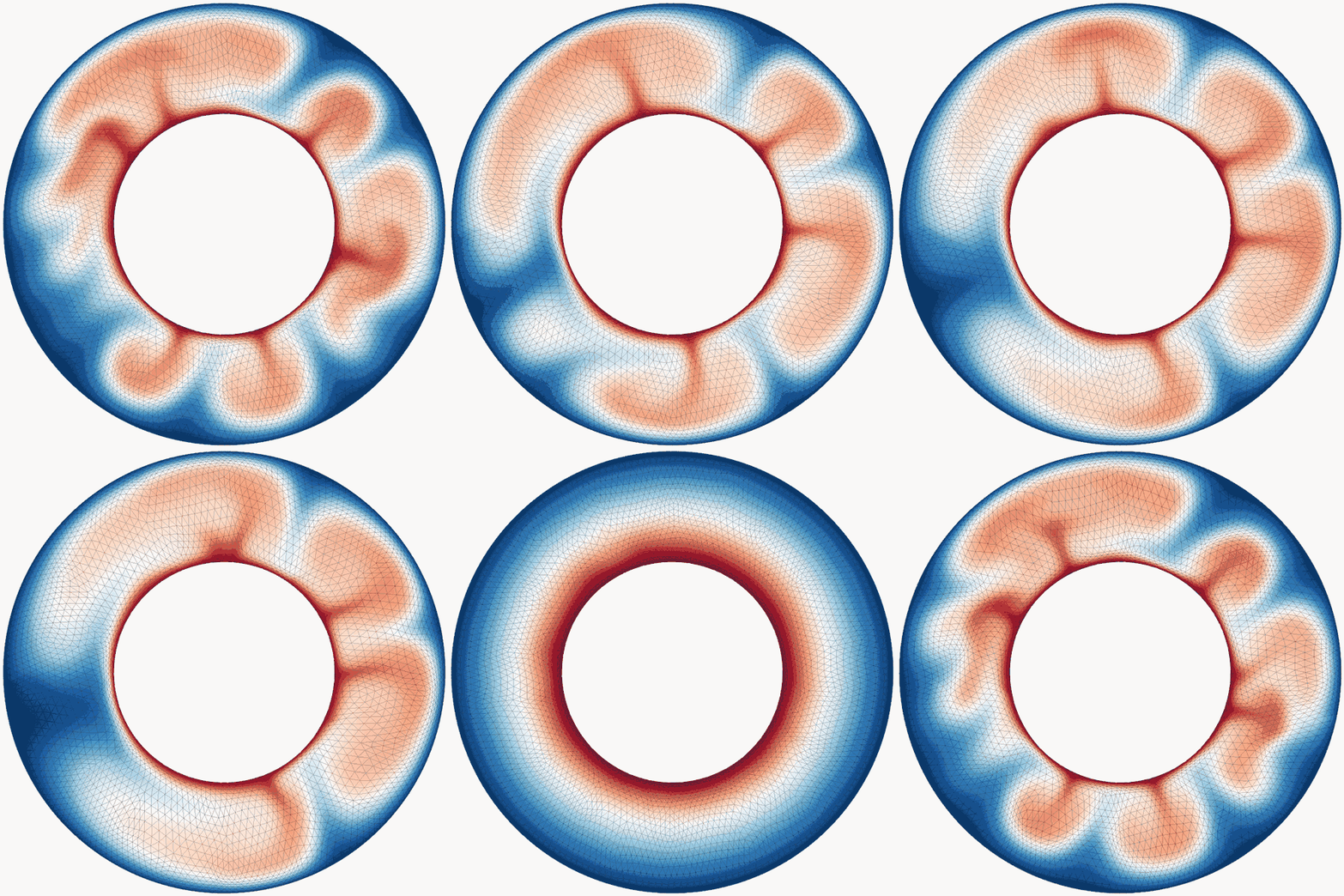
Thermal convection in an annulus with a Frank–Kamenetskii viscosity spanning a factor of 103, at defined on the lowest viscosity. The base mesh is resolution 32, and the metric asks for cells up to 8× finer than the background spacing — more than a fixed node budget can deliver, for the reason given above. The node count never changes: the mesh tightens onto the boundary layers and the plume margins and slackens in the interior, and it keeps doing so as those features migrate. Nothing here is remeshed, and the multigrid hierarchy the solver uses is the one the mesh started with.
Using it
# Redistribute to a metric, in the mesh's own reference frame.
mesh.redistribute_nodes(metric)

# Repair element shapes at fixed size, in the ideal frame.
mesh.relax()
Both keep the vertex count, the degree-of-freedom layout and the parallel partition exactly as they were.
- Huang, W., & Kamenski, L. (2015). A geometric discretization and a simple implementation for variational mesh generation and adaptation. Journal of Computational Physics, 301, 322–337. 10.1016/j.jcp.2015.08.032
- Huang, W., & Kamenski, L. (2017). On the mesh nonsingularity of the moving mesh PDE method. Mathematics of Computation, 87(312), 1887–1911. 10.1090/mcom/3271