In this article, we will see how the underworld3 sympy formulation combined with the PETSc finite element, strong-form framework builds model derivatives which can solve non-linear problems using a Newton method. This requires us to calculate the local derivative of the model with respect to the unknowns so that we know the direction to move towards a better solution.
If we differentiate the prediction a model makes with respect to one of its parameters, then we can determine how sensitive the prediction is to changes in that parameter and therefore whether the model can be used to constrain the value of that parameter. Similarly, model derivatives are used in data assimilation to determine how to adjust a model’s parameters so it better fits the observations we have 12.
The forward problem, solved by Newton
Underworld3 starts from the strong form of the equations which is usually how they are written in a textbook or a paper. These are symbolic, sympy objects that pass directly to compiled objects in PETSc 34: everything inside a divergence term goes into the flux , everything else into the force . The discrete solution is written in the finite-element basis, , and the weak form is one equation for each basis function : the integral of the two templates against it and its gradient,
, the residual (1), is the out-of-balance force: what the assembled system has left over when the current is put into the governing equation. A solution is a that makes it vanish. Here is a set of parameters of the model (for example a Rayleigh number, or a constitutive modulus) that the user typically would adjust to run an example.
A Newton non-linear solver needs the derivative of with respect to the unknowns 5:
which underworld computes directly from sympy, compiles and registers with PETSc. The Jacobian is the derivative of each equation with respect to each nodal unknown . Since and , the chain rule turns the four blocks into , assembled element by element,
, assembled by (3), is the tangent stiffness matrix. For a linear problem it is just the stiffness matrix, and
For a nonlinear problem, is the stiffness of the material at the current solution state. Newton uses it to reduce the out-of-balance force: expanding and asking for the left side to vanish gives the correction
repeated until is zero to the tolerance asked for. For a linear problem (4) makes the expansion exact, and one step gives the solution.
The adjoint problem
Now suppose we want to choose the parameters so that the model reproduces some observations as well as it can. The observations are values — a surface velocity at a station, or a stress at a point — and the model predicts the same quantities, , from its solution. The quality of the fit is the misfit
and the task is to minimise this by adjusting , under the constraint that always solves the model: at every we try. To do that we need the gradient (which way, and how far, to move each parameter) and the adjoint approach provides this for all the parameters at once - at the expense of one additional linear solve.
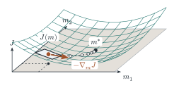
Figure 1:The misfit as a surface over two parameters (in this case). A forward solve locates the model at one point on this surface. The adjoint solve gives the tangent plane at that location. Following the gradient downhill reaches , where the model best fits the observations.
The constraint is added to the minimisation with a Lagrange multiplier 6:
which equals for any whenever the model is solved, because there. We are free to choose , and we choose it so that does not change, to first order, when the solution changes: . Transposed, that is the adjoint problem,
a linear solve for a field on the same mesh as . It is linear because is already known: and are evaluated at the converged solution and held fixed, and appears only multiplied by them. The operator is the tangent stiffness at that solution, transposed. The force is the misfit’s derivative with respect to the solution,
one entry per nodal unknown: each misfit , placed at the nodes its prediction depends on. This is the misfit written as a force, assembled like any finite-element force vector, and it is the only place the observations enter. With chosen this way, the solution’s response to drops out of , and what is left is the gradient for each parameter,
where is a pseudo-force: the out-of-balance force that appears when is nudged and the solution held still. It is an integral for each parameter, not a solve.
The appendix reaches (8) and (10) a second way, by differentiating the constraint directly, which shows what each term means.
Reducing is then a loop, Figure 2: (1) solve the model, (2) solve the adjoint problem, (3) form the gradient for every parameter, (4) update the parameters and go round again. In practice a quasi-Newton method such as L-BFGS chooses the step and builds up curvature from successive gradients.
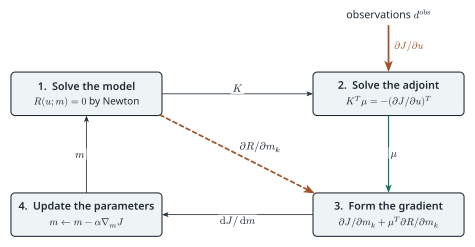
Figure 2:One pass of an inversion. Teal carries a field, rust a force, black a quantity handed on. The tangent stiffness assembled by the forward solve is the operator of the adjoint solve, and the pseudo-force comes from the same residual; the observations enter only as the adjoint’s load.
Each pass costs one nonlinear solve and one linear one, irrespective of the number of
parameters there are, and the fit improves until the gradient vanishes, at a
minimum of where no small change of brings the model closer to the
observations. The minimum may be a local one: the gradient describes the
surface only where the model is. In
Underworld3, with the misfit J written as an integrand over the mesh,
steps 2 and 3 are a single call,
dJdm = stokes.gradient(J, parameters=[m1, m2, m3])["parameters"]
dJdm[m1]                       # dJ/dm1
and step 4 is whatever optimiser one prefers.
Re-using the forward solve
The adjoint problem (8) asks for two things: the transposed stiffness , and the pseudo-force . Neither is a new object. Both are the blocks (2) that Newton already uses, read differently.
The transposed stiffness is a relabelling. is the bilinear form of (3) with trial and test exchanged. Exchanging and leaves the two diagonal terms in place, transposed on their paired indices, and swaps the two mixed ones — the term becomes a term and the other way about, with their components exchanged:
So the adjoint operator is assembled from the same four compiled kernels, registered in a different arrangement. We do that wherever the kernels carry the whole operator, rather than transposing an assembled matrix, which matters for Stokes, where the and blocks exchange places by the same rule and the composite operator stays a composite operator the Krylov solver can be preconditioned against. Nothing is differentiated a second time, and the assembled operator agrees with the explicit transpose to machine precision.
The parameter derivative is the same diff, on a different symbol.
A named quantity — a friction coefficient, a reference viscosity, a
continuation parameter — survives into and as a symbol,
because the solver carries the constitutive model’s own expression rather than
the number it currently holds. Differentiating (1) with respect
to instead of is the same operation that produced (2):
Accuracy of the gradient
Three things decide the accuracy of the gradient. The forward solve must be converged before the adjoint is taken, because is the multiplier for the constraint and has meaning only where that holds. The adjoint solve itself can be run to a loose tolerance: every pass re-solves the forward problem and recomputes , so a direction that is slightly off costs an extra iteration and the next misfit shows whether it helped. And the matrix must be the true derivative . With a frozen-viscosity Picard matrix, solves its own equation exactly and the gradient it gives belongs to no function, so the optimiser can stop where the true gradient is still large. The tangent is a property of the code rather than of the iterate, so it is checked once, by finite differences, and assembling it symbolically from the same residual is what makes it right by construction.
Derivation of the adjoint
The adjoint problem (8) and the gradient (10) also follow from differentiating the constraint directly, without the Lagrangian (7), and this route shows what each term means.
We explicitly wrote in terms of to demonstrate that there is an entire family of solutions to that we can access by changing the model’s free parameters. If the model makes a prediction, , we can ask how changing affects that prediction (the sensitivity of the prediction to ). That is
If is an underworld function then we can form a symbolic expression. First we note that and are not independent: the solution is constrained to the family of solutions of (1), holds for every and, because of this, is zero too
The first factor is the tangent stiffness again, so
is the pseudo-force of (10): the out-of-balance force that appears if the parameter is nudged and the solution is held still. It is assembled exactly as is, with and in place of and .
We interpret (15) as: the sensitivity of the solution to a parameter is the response of the structure to that parameter’s pseudo-force.
The prediction depends on in the same two ways: directly, and through the solution. With the row of derivatives with respect to the nodal unknowns — the prediction written as a force — the chain rule and (15) give
Many parameters at once
A real model has many parameters, , and we want the sensitivity for all of them. We first write (16) like this:
These are equations that differ only in their last factor, the pseudo-force . The row in front of it, , contains the prediction and the stiffness but no parameter; it is the same for every and we only need to compute it once.
Now define through
We do not have access to so we multiply both sides by on the right, take the transpose and substitute into (17) to recover (8):
One linear solve for , whatever is, and then one product for each parameter. Written as fields, with , that product is
which is the pseudo-force’s weak form with in the place of the test function.
, the adjoint state, is the response of the same structure to the misfit’s force: an influence field, in the sense of an influence line. It says how strongly an out-of-balance force applied anywhere in the domain would tell on the misfit. With it in hand, the derivative for a parameter is — the virtual work that parameter’s pseudo-force does against the influence field — and that is an integral, not a solve.
Solving (15) for each and contracting it with gives the same numbers, at the cost of solves. That the two agree is Maxwell–Betti reciprocity: the work done by one force through the displacements of another equals the work done by the second through the displacements of the first. The transpose is what makes it true for a problem whose stiffness is not symmetric.
So the adjoint is cheap in parameters and dear in misfits. One solve for ten parameters or a thousand; another solve for every additional misfit. That suits a model with many dials and one thing you care about, which is the usual shape of the problem.
One stiffness, three forces
The Newton update, the forward sensitivity and the adjoint are three linear solves with the same matrix and different right-hand sides:
Newton has already assembled and preconditioned that matrix, so the adjoint costs one more linear solve.
The Underworld project is supported by AuScope and the Australian Government through the National Collaborative Research Infrastructure Strategy (NCRIS). Source code: github.com/underworldcode/underworld3
- Bunge, H.-P., Hagelberg, C. R., & Travis, B. J. (2003). Mantle circulation models with variational data assimilation: inferring past mantle flow and structure from plate motion histories and seismic tomography. Geophysical Journal International, 152(2), 280–301. 10.1046/j.1365-246x.2003.01823.x
- Liu, L., & Gurnis, M. (2008). Simultaneous inversion of mantle properties and initial conditions using an adjoint of mantle convection. Journal of Geophysical Research: Solid Earth, 113(B8), B08405. 10.1029/2008jb005594
- Moresi, L., Mansour, J., Giordani, J., Knepley, M., Knight, B., Graciosa, J. C., Gollapalli, T., Lu, N., & Beucher, R. (2025). Underworld3: Mathematically Self-Describing Modelling in Python for Desktop, HPC and Cloud. Journal of Open Source Software, 10(112), 7831. 10.21105/joss.07831
- Knepley, M. G., Brown, J., Rupp, K., & Smith, B. F. (2013). Achieving High Performance with Unified Residual Evaluation. 10.48550/arXiv.1309.1204
- Moresi, L., Mansour, J., & Giordani, J. (2026). How Underworld3 Turns SymPy into C. figshare. 10.6084/m9.figshare.33193572
- Plessix, R.-E. (2006). A review of the adjoint-state method for computing the gradient of a functional with geophysical applications. Geophysical Journal International, 167(2), 495–503. 10.1111/j.1365-246X.2006.02978.x