Underworld Release 2.8

Version 2.8 of Underworld has been released recently. As with all major releases, this release brings numerous new features, enhancements and bug fixes. A summary of changes may be found within the usual CHANGES.md file. As is also usually the case, numerous API changes have been necessary or warranted. Most significantly, this release marks a departure from Python2 compatibility, with this and all future releases moving exclusively to Python3 operation.

In this post we’ll consider the following:

1. The move to Python3
2. The Semi-Lagrangian Advection Diffusion Scheme
3. Improved Particle Data Querying
4. Collective HDF5 IO
5. API Changes
6. How To Update

Note that all example notebooks in this post include links to live instances so you can test out the new functionality yourself. Just click the LIVE DEMO link under each example. Thanks to the folks at  Binder for providing the cloud compute!

The move to Python3

The switch to Python3 has been motivated by a number of factors. Most pressing is the scheduled end of life for Python2 set for the end of this year. While Python2 will no doubt still be in use for the foreseeable future, it will no longer be officially maintained, and there will be no Python version 2.8. As an actively developed Python project, it is necessary that we move with the community in adopting Python3 as the new de facto standard for Python. This will ensure our future viability as third party libraries we utilise also switch to Python3. Perhaps more importantly, we reduce the risk of exposing our users to security vulnerabilities that may arise when using outdated software.

Further to this, the limitations of Python2 resulted in some difficulties with usage of the Underworld API. Specifically, our usage of metaclasses broke autocomplete and tooltip suggestions within the Jupyter environment, functionality that is critical to frictionless development of Underworld models (or usage of any Python API for that matter). Python3 introduces the signature() function to the inspect module, allowing us to restore the required class constructor signatures. Python3 also includes many other improvements (type hinting, better maths handling, etc) that we will eventually utilise within the UW API.

While it is possible to simultaneously support both Python2 and Python3, we have decided for simplicity to discontinue Python2 support. This minimises the complexity of maintaining  our API, allowing us to instead focus on improving core functionality. Any changes which breaks backwards compatibility are not taken lightly, though in this instance it is felt that for most users updating Python3 should be relatively trivial. There are two steps required for the switch to Python3:

1. Installation of a Python3 interpreter.
2. Update your models for Python3 compatibility.

As most of our users utilise Docker for their Underworld environment, no explicit action is required for the first step. Updating to Underworld 2.8 only requires pulling down our latest release image, and the Python3 interpreter is included within the image. For other users who have locally compiled versions of Underworld, naturally they will need to have a Python3 interpreter installed if one is not already available. For HPC usage, we have updated instructions available for the commonly used platforms. As always, if you have difficulties, please do not hesitate to raise an issue on our GitHub issue tracker.

The second step required for the switch involves updating your models to reflect the various syntax and API changes Python3 introduces. This will apply for all users, but generally should only involve trivial changes. We cover the changes you are likely to require in the following section.

Python3 Changes

For most users, only superficial changes will be required for Python3 amenability. Indeed for many, it will simply be a case of switching from using print statements (deprecated in Py3) to print() functions. So where you previously have written:

>>> print "Hello, World! 

Hello, World!

you will now need:

>>> print("Hello, World!)

Hello, World!

The other change we’d like to highlight is the way in which Python3 handles division arithmetic. In Python2 division between two integers always result in a truncated integer, although if either argument is a float then floating point division will occur:

>>> 3/2
1
>>> 3.0/2
1.5

For Python3, all division using the / operator is floating point division:

>>> 3/21.5
1.0
>>> 3./21.5
1.5

It is unlikely that you rely on the Python2 behaviour, but we wish to flag this in particular as it may lead to changes in your models that go unnoticed (unlike the print changes which will immediately raise an error). If you wish to use integer division, both Py2 and Py3 support the // integer division operator, and also satisfies the Python ethos of explicit is better than implicit.

For further information on the differences between Python2 & Python3, you may like to review this page.

The Semi-Lagrangian Advection Diffusion Scheme

The Semi-Lagrangian Crank-Nicholson (SLCN) algorithm, a numerical method for solving the advection diffusion equation, is now available in the 2.8 release.
SLCN is an alternative to the Streamline Upwind/Petrov-Galerkin (SUPG) algorithm that Underworld currently provides for the finite element method modelling of a scalar field evolving under the processes of advection and diffusion (traditionally  used for the heat equation in Underworld).

The advantages of SLCN over SUPG:

• Less numerical diffusion.
• Unconditionally stable, allowing larger time-steps.

The method, proposed by Spiegelman and Katz², performs well over a large range of Péclet numbers, including the end members: zero diffusion or pure diffusion. In addition, the method is not constrained by a CFL stability condition, and therefore the user is free to use arbitrarily large step sizes. Naturally, the length scales you wish to resolve accurately will still place a limit on the step size. For benchmarking purposes, the venerable, well-characterised SUPG solver will still be available in future releases.

To switch to the new SLCN method, set the method attribute when defining the AdvectionDiffusion class, i.e.

import underworld as uw
### domain and field initialisation
advDiff = uw.system.AdvectionDiffusion( ... , method='SLCN', ... )

Note that if the method parameter is not specified, the class will default to the SUPG scheme. This gives the expected behaviour for backwards compatibility, and allows for a grace period having SLCN being used and tested in the wild. In the future the default behaviour may switch to using the SLCN scheme.

Looks great, right ?  Here’s the notebook for the above simulations:

You can run a live demo of this notebook on mybinder.org

That said the current implementation is not perfect. For models with non orthogonal meshes or periodic boundary conditions the implementation is slow or broken respectively. Development to fix these usage restrictions will be released in future Underworld versions.

To summarise, SLCN is generally a superior method for modelling advection-diffusion processes, yielding less numerical diffusion for high Péclet number models, and enabling larger time-step sizes than the SUPG counterpart.

Improved Particle Data Querying

For a long time now, particle swarms within Underworld lacked all the functionality of their Eulerian brethren. Specifically, it was not possible to query particle swarms at arbitrary locations in space. This severely limited the application of the evaluate() method, which could only evaluate particle based data en masse across the entire swarm, at each and every particle’s location. This is generally heavy operation, but also wasn’t useful if the user wanted to obtain values a certain locations of interest (along a line or interface perhaps). It was also inconsistent with the behaviour of mesh data objects, which could indeed be interrogated at arbitrary coordinates.  In the case of mesh data objects, a natural path for this is provided via the finite element interpolation functions which are used to form a weighted average result. In our usage however, particle data is purely discrete, which therefore begs the question: what value do we return at an arbitrary coordinate? In the first instance, the answer to this will be to simply return the value of the nearest corresponding particle. For efficient nearest neighbour (NN) searching a k-d tree algorithm is utilised, with the implementation provided via the excellent nanoflann library.

Let’s take a look at simple example:

You can run a live demo of this notebook on mybinder.org

In the above demo, we simply add particles along with a swarm variable which records their local index. We then query this index variable at a coordinate for which we know which particle is expected to be closest, and confirm the result.

Since swarm variable objects can now be queried at arbitrary coordinates, we are also able to use them for visualisation using the Surface drawing object, or anywhere else where a Function object is expected to respond to a global coordinate:

A live demo is available on mybinder.org

There are numerous caveats to usage of this new particle querying behaviour. Firstly, it can only currently be used for analytics and visualisation, and not within the underlying finite element matrix construction. Actually, the finite element problem already uses a NN algorithm for the mapping of particle data to Gauss points¹, however this algorithm requires that each element has at least a single particle within it. Secondly, parallel operation is still experimental and identical results to serial operation is not guaranteed. This is due to the fact the NN searching will only consider the local domain of each process. Where your swarms are sufficiently dense, such that the neighbour nearest to the query location is on the local process, the correct behaviour will ensue. By default, an error will be trigger if you try use NN in parallel, though you may optionally suppress this if you wish to continue.

In the future we hope to allow the usage of NN behaviour dynamically, such that a sparse swarm may be utilised to represent your materials. We also intend to introduce interpolation routines to extract values using weighted averages of particles neighbouring the query locations.

Collective H5 IO

For large parallel simulations, data IO operations can quickly begin to dominate wall time. While previous version of Underworld collectively opened and closed files to avoid filesystem locking, the data writing itself was essentially a serial operation. This is reflected in the graph below, with total write times tracking with job size (dashed line).

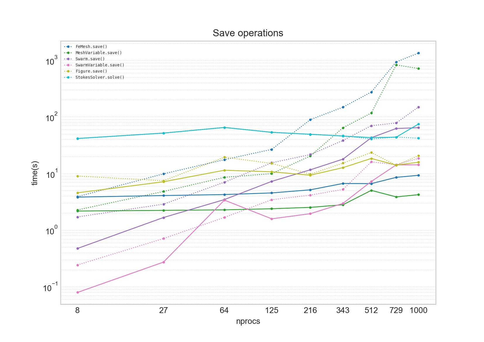
Indeed disk write time (for the mesh) exceeds system solve time (light blue line) for jobs of greater size than 216 processes. In Underworld v2.8, dramatic improvements in write times have been achieved by enabling collective writing via h5py (shout out to Rui@NCI for flagging this to us!). For mesh objects, collective writing results in a flattening of the timing curves, with a two orders of magnitude improvement observed for the largest simulations. The picture was less clear for swarm objects however, with resulting write time changes being neither here nor there. This is due to the differences in writing patterns for particle and mesh data. We hope to make further improvements for writing swarm objects in future releases.

Collective writing is enabled in UW2.8 for mesh objects, and optional for swarm objects (defaults to off). As always, we urge users to minimise their requirement for writing data to disk, and instead where possible perform analytics inline within their simulations scripts. Obviously writing to disk incurs a time overhead, but there is also the associated burden of file handling which for large datasets becomes non-trivial. For very large simulations, inlined analytics may be the only viable option.

API Changes

The mpi submodule

Routines to extract MPI related information is now located in the underworld.mpi submodule. You will require the following changes:

• underworld.nProcs() → underworld.mpi.size
• underworld.rank() → underworld.mpi.rank
• underworld.barrier() → underworld.mpi.barrier()

Note above that rank and process count information is now accessed as module attributes. We have also introduced the underworld.mpi.call_pattern() context manager which is useful for forcing sequential operation where required.

GlobalSpaceFillerLayout is now deprecated

The GlobalSpaceFillerLayout was effectively serial in operation, and therefore quickly became a bottleneck for parallel simulations. As such, it has now been retired in favour of the parallel friendly PerCellSpaeFillerLayout which provides very similar layouts. Update your models accordingly.

How To Update

We have published new release images to our DockerHub page. Note that the docker latest tag is always aliased to the most recent stable build image (so currently 2.8.1b). Kitematic users will need to create a new container which should then pull  down latest image (remember to check your volume mapping settings are correct). Those comfortable at the command line can run docker pull underworldcode/underworld2 to pull down the new image. As mentioned earlier, Python3 is already included in the release image

For users creating native builds, you should obtain the latest repository via git clone or git pull, and then follow the usual compilation process. Remember that you will need to have a Python3 interpreter installed. You may like to consider using virtualenv if you wish to concurrently have access to Python2 and Python3 environments.

For HPC, users will either need to create a new native build of Underworld 2.8, or, where possible, use containered alternatives. For Pawsey-Magnus, the standard Underworld image is compatible with their Shifter container environment, and you may therefore simply pull down the latest image and run immediately. Please refer to the Pawsey Shifter documentation for usage instructions.  TACC-Stampede2 currently has experimental support for containers via Singularity, although you will need to use the custom image we have created which is tagged 2.8.0b_stampede2_psm2 (usage instructions are available here). Compilations instructions for various platforms is available within our github repo.

1. A Voronoi algorithm is also available, though is not used by default (See Velić, M., D. May, and L. Moresi. “A Fast Robust Algorithm for Computing Discrete Voronoi Diagrams.” Journal of Mathematical Modelling and Algorithms 8, no. 3 (2009): 343–55. https://doi.org/10.1007/s10852-008-9097-6.)
2. Spiegelman, Marc, and Richard F. Katz. “A Semi-Lagrangian Crank-Nicolson Algorithm for the Numerical Solution of Advection-Diffusion Problems.” Geochemistry, Geophysics, Geosystems 7, no. 4 (2006). https://doi.org/10.1029/2005GC001073.