Abstract
As the old truism states, the best way to learn is by doing. This guide can get you from zero to hero in 60 seconds - give or take.
As the old truism states, the best way to learn is by doing.
This is terribly unhelpful since, really, you can’t ‘do’ anything until you learn. This is a Catch-22 that every grad student encounters; doubly so when it comes to anything involving code, where daily life provides very little in the way of intuition.
Unlike other geodynamic modelling software, Underworld is designed to be approached with code. The downside is that the learning curve starts with a bump. The enormous upside is that, once you have a little fluency under your belt, you will find your science moves at the speed of thought.
But how do you surmount that bump?
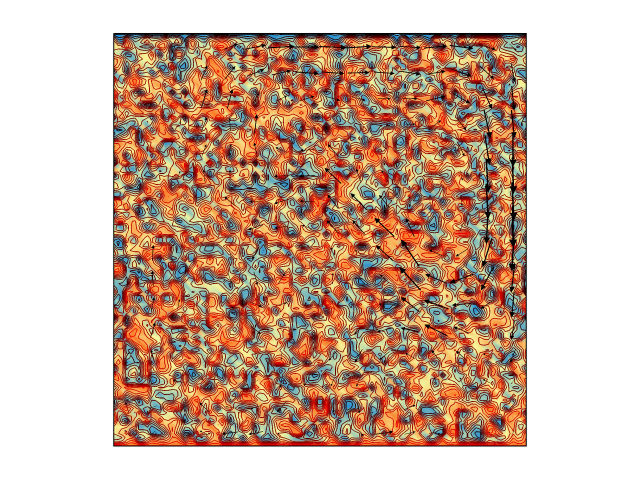
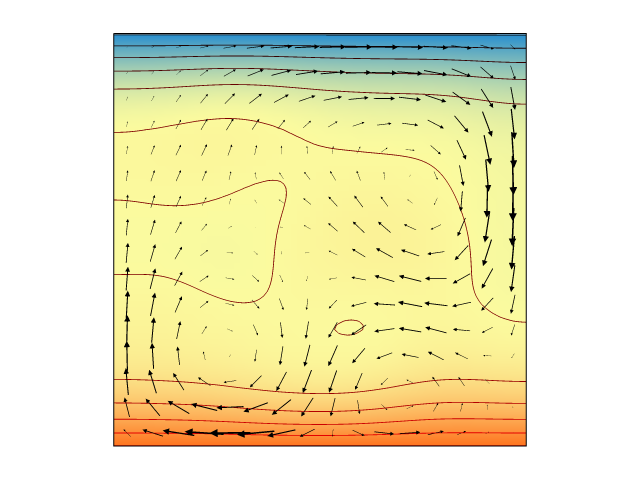
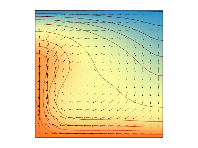
If all goes well, this is where you’ll be five minutes from now!
Preparing your workspace
In this short how-to, we’re going to lay out a 60-second scheme to get you up and running in Underworld. But before we start, we’ll need to make sure you’ve got the right tools.
You will need:
A computer. Although Underworld is proudly Turing Complete, hand iteration is not recommended.
A terminal. On Windows this might be PowerShell or Command Prompt; on Mac and Linux it’s just called the Terminal. In any case what you’ll get is a blank background with a blinking cursor beckoning you to type your bidding into the computer.
A working instance of Docker. Docker supports containers which are like mini-computers that live inside a bigger computer. If you’re new to containers, try Docker Desktop: get started here.
A browser. We recommend Chrome for ease of use or Firefox if you’re concerned about the depredations of late capitalism. Avoid Safari (both the software and the kind that involves lions).
Some place on your hard drive that you’re happy to use for Underworld stuff: a folder in your Documents, for instance. Anywhere will do so long as it’s not on a network or share drive (this could make your sysadmin unhappy). Jot down the filepath of this directory as you will need it shortly. Try to get the ‘absolute’ filepath if you can (on Windows, this will start with
C:\or similar; on Linux and Mac, simply/).
That’s it!
Tying your shoelaces
So we don’t get tripped up by any lurking gremlins, let’s quickly test to see if things are working as they should.
Open your terminal. (Try your OS’s search bar if you can’t find it)
Type in
dockerand hit enter. You should get a little introduction and a list of commands: this is everything that Docker can do for you.Type in
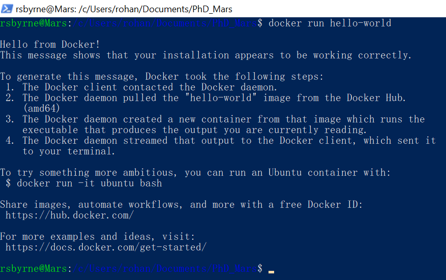
docker run hello-worldand hit enter. After a little number-crunching you should receive a cute message from the good folks at Docker Hub.
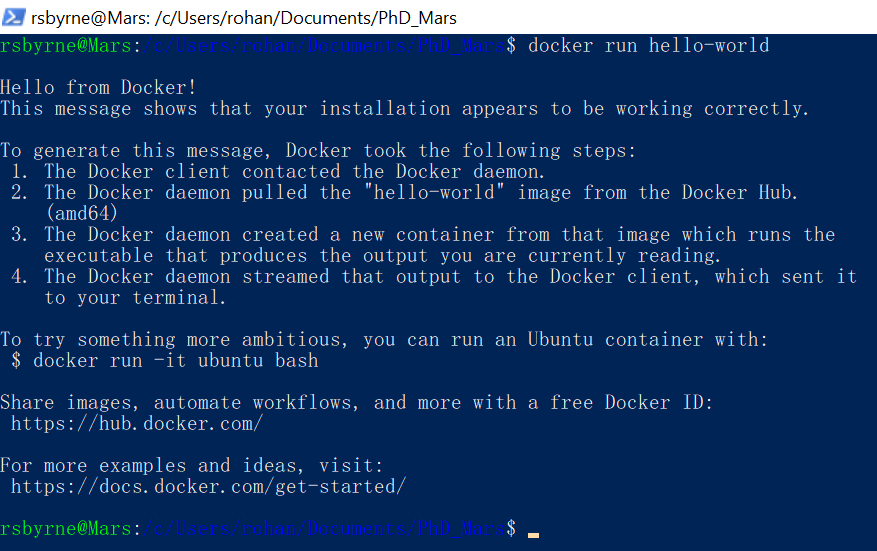
Thanks Docker !
If you get errors instead, you will have to do some good old troubleshooting. None of the rest of our guide will work unless Docker is installed and correctly configured.
But if everything looks shipshape, you’re ready to run.
On your marks...
Take a deep breath. You are about to become a champion Underworld2 geodynamic numerical modeller.
Go!
Start the clock.
Hardly seems fair...
Open your terminal
Do you have your target directory from before? You’ll need it. Type in the following docker command, where ‘YOUR_DIRECTORY’ is your nominated folder:
docker run -v YOUR_DIRECTORY:/home/jovyan/workspace/ -p 127.0.0.1:8888:8888 underworldcode/underworld2:latestStop the clock! This may take some time depending on your internet connection and whether you’ve tried it before. When it’s ready, you should get a message with a URL in it.
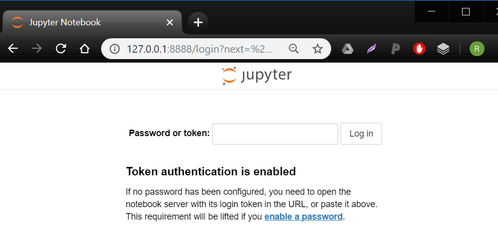
Go to your browser and type the following into the address bar:
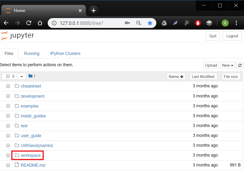
127.0.0.1:8888You may need to provide a ‘token’ to access: you can copy-paste this from the command prompt where you ran Docker just before. Consider following the prompts to set up a password, which will save you time in the future.You are now in ‘Jupyter Notebooks’, which is a browser-based environment for writing and running code. Navigate to the ‘workspace’ directory. This directory is actually the very same as YOUR_DIRECTORY - it has been ‘mounted’ into the container. Make a new file in Jupyter and you should see it pop up in the appropriate place on your desktop, and vice versa.
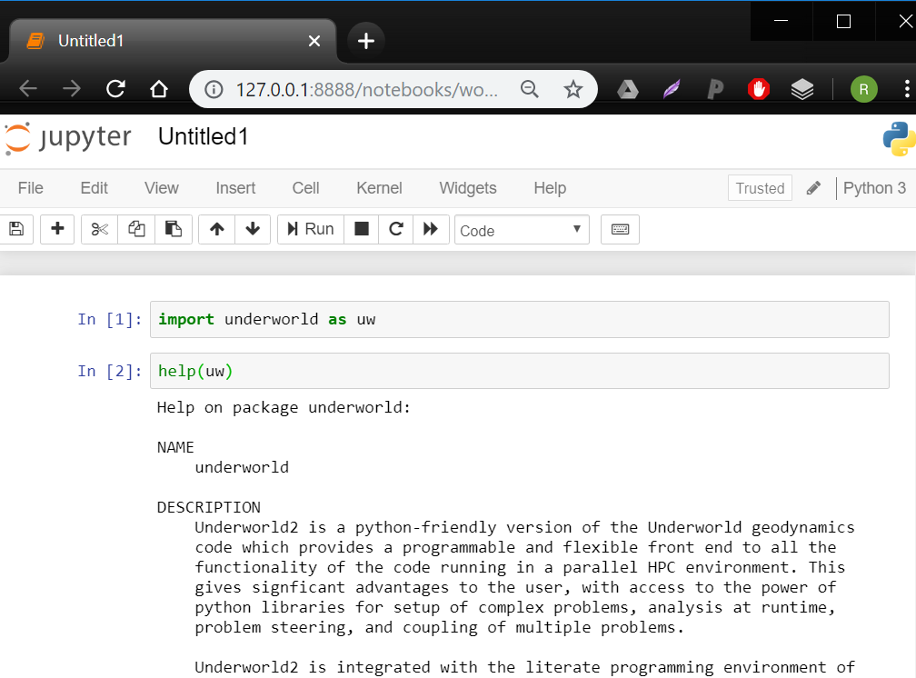
Inside ‘workspace’, click the ‘new’ dropdown button and select ‘Python 3’. It will open a new ‘notebook’ with a blank ‘cell’ at the top.
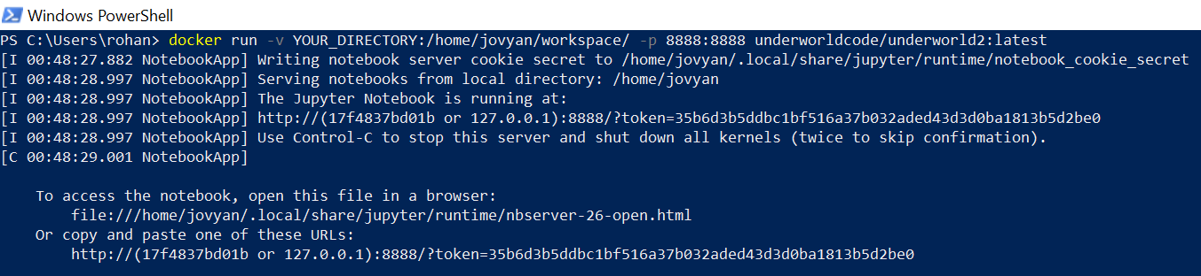
Being able to imagine a job is 9/10ths of being able to perform it (but the remaining 1/10 is what you get paid for...)
Believe it or not, you now have a fully functional geodynamic numerical modelling environment at your very fingertips!
Still time on the clock? Let’s see if we can get an actual model up and running. At the bottom of this article you will find a long code snippet. This is a complete, working, research-ready Underworld model which demonstrates the consequences of exponentially temperature-dependent rheology. Just cut, paste, and hit enter.
You could be using this for science right now: what are you waiting for?
Podium finish
If everything goes right, this guide should have taken you from Spider Solitaire to geodynamic modeller par excellence in 60 seconds. But if it didn’t, you can always get in touch with us for help. Underworld is more than just a bit of software: it’s a vibrant, passionate, and diverse research community dedicated to helping you answer your question - and have fun doing it.
Now you’ve taken the first step, try getting started on our interactive user guide, which can be found online as well as in the container itself, in the root directory. And follow our channels on Ghost, Medium, Facebook, Twitter, and GitHubfor more how-tos, tutorials, meet-ups, updates, and general research chatter.
Turns out the best way to learn really is by doing. But that doesn’t mean you have to do it alone.
-Rohan
# MY FIRST MODEL:
# ARRHENIUS RHEOLOGY IN UNDERWORLD
'''
Cut and paste me into one or more cells
of you Jupyter notebook and hit enter.
Or save as a script and execute from terminal
with:
mpirun -n 4 python YOUR_SCRIPT.py
...to execute in parallel on four cores.
Change the parameters to investigate
the impact of varying degrees of
temperature-dependent viscosity.
'''

import numpy as np

import underworld as uw
fn = uw.function
import glucifer

# Define physical parameters:
Ra = 1e7
eta0 = 3e4
res = 64

# Create the computational mesh:
mesh = uw.mesh.FeMesh_Cartesian(
    elementRes = (64, 64)
    )

# Create the system variables:
temperatureField = mesh.add_variable(1)
temperatureDotField = mesh.add_variable(1)
pressureField = uw.mesh.MeshVariable(mesh.subMesh, 1)
velocityField = mesh.add_variable(2)

# Define the walls:
inner = mesh.specialSets["MinJ_VertexSet"]
outer = mesh.specialSets["MaxJ_VertexSet"]
left = mesh.specialSets["MinI_VertexSet"]
right = mesh.specialSets["MaxI_VertexSet"]

# Define boundary conditions along the walls:
tempBC = uw.conditions.DirichletCondition(
    variable = temperatureField,
    indexSetsPerDof = (inner + outer)
    )
velBC = uw.conditions.DirichletCondition(
    variable = velocityField,
    indexSetsPerDof = (left + right, inner + outer)
    )

# Define the laws of physics:
buoyancyFn = Ra * temperatureField * (0., 1.)
viscosityFn = fn.math.pow(
    eta0,
    1. - temperatureField
    )
heatingFn = 1.
diffusivityFn = 1.

# Create the mathematical systems that solve them:
stokes = uw.systems.Stokes(
    velocityField = velocityField,
    pressureField = pressureField,
    conditions = [velBC,],
    fn_viscosity = viscosityFn,
    fn_bodyforce = buoyancyFn
    )

solver = uw.systems.Solver(stokes)

advDiff = uw.systems.AdvectionDiffusion(
    phiField = temperatureField,
    phiDotField = temperatureDotField,
    velocityField = velocityField,
    fn_diffusivity = diffusivityFn,
    conditions = [tempBC,]
    )

# Define the basic running constants:
step = fn.misc.constant(0)
modeltime = fn.misc.constant(0.)

# Make a function to initialise the model:
def initialise():
    step.value = 0
    modeltime.value = 0.
    randArray = np.random.rand(*temperatureField.data.shape)
    temperatureField.data[...] = randArray
    temperatureField.data[outer] = 0.
    temperatureField.data[inner] = 1.
    solver.solve()

# Create a figure so we can see what's happening:
fig = glucifer.Figure()
fig.append(
    glucifer.objects.Surface(
        mesh,
        temperatureField,
        colourBar = False
        )
    )
fig.append(
    glucifer.objects.VectorArrows(
        mesh,
        velocityField
        )
    )
fig.append(
    glucifer.objects.Contours(
        mesh,
        fn.math.log2(viscosityFn),
        colours = 'red black',
        colourBar = False
        )
    )

# Make a convenience function for the figure:
def show():
    if uw.mpi.rank == 0:
        print('step: ', step.value)
        print('time: ', modeltime.value)
    fig.show()

# Let's have a look at what we've got:
initialise()
show()

# Make a function that iterates the model:
def iterate():
    dt = advDiff.get_max_dt()
    advDiff.integrate(dt)
    solver.solve()
    step.value += 1
    modeltime.value += dt

# Make a convenience function for multiple iterations:
def go(n):
    for i in range(n):
        iterate()

# Let's go!
for i in range(100):
    go(10)
    show()