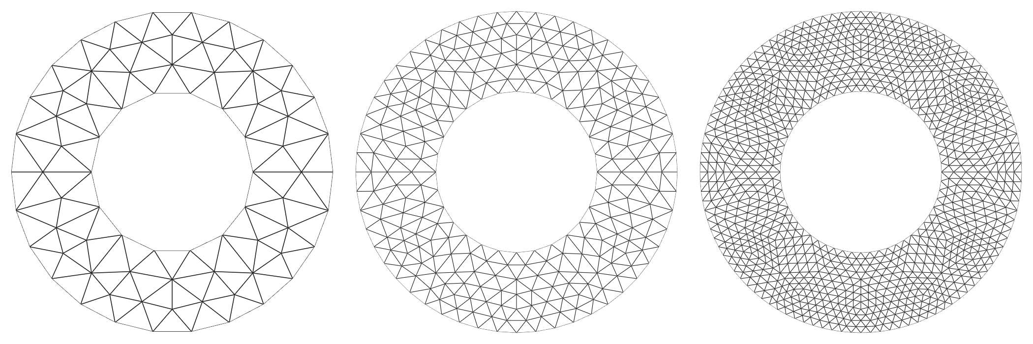
Most of the effort in a geodynamics model goes into solving the Stokes equations, and most of that is spent on the velocity solver. How that solver is preconditioned sets how long a model takes to run. Multigrid methods accelerate elliptic solvers using a hierarchy of mesh resolutions. Underworld can build the preconditioner from a real hierarchy of meshes or directly from the matrix alone, and this note is about how to build that hierarchy and what it is worth.
What multigrid does
An iterative solver reduces error unevenly. Simple relaxation methods (smoothers) are good at removing error that varies rapidly from cell to cell, and poor at removing error that varies smoothly across the whole domain. The smooth part is then what costs: it takes many sweeps to carry information from one side of a fine mesh to the other.
Multigrid turns that around. Error that is smooth on a fine mesh is not smooth on a mesh twice as coarse, where it spans half as many cells, so a few sweeps there can quickly reduce error that the fine grid struggles with.
The method is a recursion on that idea: smooth on the fine mesh, transfer what is left to a coarser one, solve there with another recursive step, transfer the correction back, smooth again. Each level handles the band of error it can see, and the work per unknown flattens out as the model gets bigger.
The two things we need: the coarse levels, and the operators that move between them.
Two ways to build the coarse levels
Algebraic multigrid (AMG) builds the coarse levels from the matrix representation of the problem directly. It inspects the operator’s connectivity, groups unknowns that are strongly coupled, and constructs coarse representations and transfer operators from that grouping alone. Because it asks nothing of the mesh, it works everywhere. PETSc’s implementation is GAMG, and it is what Underworld uses by default.
Geometric multigrid (GMG) uses actual coarser meshes. If the fine mesh was built
by refining a coarse one, those coarser meshes already exist, and the transfers
follow from the refinement relation: each fine node either coincides with a
coarse node or lies inside a known coarse cell. In PETSc this is pc_type=mg,
and Underworld runs it as a full multigrid cycle: solve on the coarsest mesh,
interpolate that solution up to the next mesh as a starting point, and repeat,
cycling up and down through the levels at each stage to clear the error the
interpolation leaves behind. We’ll refer to this as FMG.
The difference between them shows up when the operator’s connectivity is a poor guide to the geometry, which can happen when there are jumps or steep gradients in material properties. The algebraic method sees a matrix whose couplings are dominated by the stiff region and groups unknowns accordingly; the geometric method uses the grids it was given and is indifferent to the coefficients. Which of those is the better bet is not obvious in advance, so we’ll measure it and see what works. Switching the geometric solver on comes first, and we start with the hierarchy of meshes.
Making a mesh with a hierarchy
A mesh only carries a hierarchy if it was built with one. That is the
refinement argument:
mesh = uw.meshing.UnstructuredSimplexBox(cellSize=0.05, refinement=2)
len(mesh.dm_hierarchy)     # 3: the base and two refinements
The mesh you get back is the finest level, and the coarser ones are stored
within it as PETSc DMPlex objects in mesh.dm_hierarchy. Those are what the
preconditioner uses. They are not Underworld meshes, there is no Mesh object
for a coarse level, and making one takes work. The hierarchy is something
the solver knows about rather than something you handle.
Build the same mesh at cellSize=0.0125 with no refinement and you get about
the same resolution with no hierarchy at all, and so no geometric multigrid.
Algebraic multigrid runs perfectly well on a mesh that has a hierarchy; it just
does not use it.
The solver picks it up on its own:
stokes = uw.systems.Stokes(mesh)
stokes.solve()                       # preconditioner defaults to "auto"

stokes.preconditioner = "fmg"        # or "gamg", or back to "auto"
stokes.solve()
"auto" uses geometric multigrid when len(mesh.dm_hierarchy) > 1 and GAMG
when it does not. You can also ask directly, with "fmg" or "gamg". Two
behaviours are deliberate: "auto" only ever adds geometric multigrid to an
untouched configuration, so it will not overwrite preconditioner options you
have set yourself; and where a request cannot be honoured, you can find the
reasoning in stokes.pc_fallbacks. stokes.preconditioner_settings reports
what was actually applied.
Curved boundaries need help
Refining a mesh puts new nodes at the midpoints of existing edges. On a straight boundary that works well. On a curved one it is not enough: the coarse mesh approximates a circle by a polygon, and the midpoint of a chord lies inside the circle rather than on it. Those midpoints have to be moved back onto the boundary each time the mesh is refined.
Underworld’s curved meshes carry a refinement callback that snaps
boundary-labelled nodes back onto the true surface after each refinement. For
the annulus it is a few lines: take the nodes labelled Upper and Lower and
rescale each to the correct radius:
coords[upper] *= radiusOuter / R[upper]
coords[lower] *= radiusInner / R[lower]
This happens automatically for the built-in meshes, so in normal use there is nothing you need to do. It does matter if you build a mesh of your own with curved boundaries: without a callback of this kind, the finest mesh still has the coarsest mesh’s faceting, and the boundary it represents is the polygon rather than the circle.
What the coarse mesh leaves behind
Because the fine mesh is made by subdividing the coarse one, the coarse mesh’s own triangulation is still visible in it. Its edges survive as continuous lines across the fine mesh, and its vertices remain places where an unusual number of elements meet and the element density is inherited from the coarse triangulation.
mesh.relax() moves the nodes to improve element shapes while keeping the
resolution and the topology, and it helps to loosen that imprint.
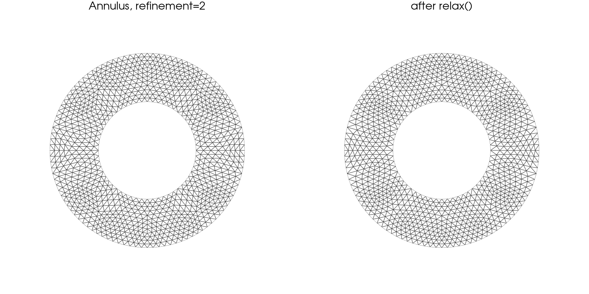
A twice-refined annulus, before and after relax(). The seams on the left are
the coarse mesh’s own edges, still visible after two refinements. Median
element quality goes from 0.940 to 0.972 and the tenth percentile from 0.839 to
0.927; the worst single cell goes the other way, 0.827 to 0.763, because the
mover minimises a global energy and will trade a few cells for many. Every node
that began on a bounding circle is still exactly on it: relaxation moves
interior coordinates only.
Relaxation moves coordinates but not topology, so the refinement relation between the levels is untouched and the hierarchy survives it. Moving a mesh without rebuilding it is the subject of a related technical note.
When the choice matters
The test is SolKz, a standard Stokes benchmark on the unit box: viscosity
varying exponentially with depth, , forced by
with , , free slip
on all four walls, Taylor–Hood – elements. The viscosity contrast
across the box is . SolKz has a closed-form solution, and Underworld
carries it in uw.analytic — putting it to its usual use, checking that a
solver converges to the right answer, is the subject of a
companion note. Nothing here uses
it: these are cost measurements, not accuracy measurements.
Computational work is reported as floating-point operations (counted by PETSc) per unknown and relative to the constant-viscosity FMG run with a fixed target iteration tolerance across the board. Flops are a useful measure: they do not depend on the machine, and they are generally deterministic. Times are given alongside, because they are what you wait for and they reveal that different algorithms may be more or less efficient on particular hardware.
First we examine the cost against viscosity contrast, at 11 727 unknowns:
| preconditioner | viscosity contrast | relative work per unknown | relative time per unknown |
|---|---|---|---|
| FMG | 10⁰ | 1.0 | 1.0 |
| FMG | 10² | 1.3 | 1.1 |
| FMG | 10⁴ | 1.6 | 1.2 |
| FMG | 10⁶ | 1.8 | 1.3 |
| GAMG | 10⁰ | 2.2 | 1.2 |
| GAMG | 10² | 3.3 | 1.5 |
| GAMG | 10⁴ | 4.0 | 1.7 |
| GAMG | 10⁶ | 4.0 | 1.6 |
Both solver configurations handle the whole range in the viscosity gradient sweep and there is almost no change in the amount of work required or time taken to solve. GAMG does slightly more work but does so a little more efficiently.
Next, let us look at the cost (per unknown) as we change the problem size, at constant viscosity:
| preconditioner | unknowns | relative work per unknown | relative time per unknown | Gflop/s |
|---|---|---|---|---|
| FMG | 2 947 | 1.0 | 1.0 | 1.6 |
| FMG | 11 727 | 1.7 | 1.3 | 2.1 |
| FMG | 46 783 | 2.2 | 1.4 | 2.4 |
| FMG | 186 879 | 2.5 | 1.6 | 2.4 |
| FMG | 747 007 | 2.6 | 1.8 | 2.2 |
| GAMG | 2 947 | 2.7 | 1.3 | 3.4 |
| GAMG | 11 727 | 3.8 | 1.5 | 3.8 |
| GAMG | 46 783 | 4.0 | 1.6 | 3.9 |
| GAMG | 186 879 | 4.6 | 1.7 | 4.2 |
| GAMG | 747 007 | 5.5 | 1.9 | 4.6 |
Both flatten (which is good). Step by step, FMG’s flop count goes as , , , ; GAMG’s as , , , . Both are converging on linear, which is what multigrid of either kind is supposed to do: the algebraic method reaches it as surely as the geometric one.
So the geometric hierarchy is worth roughly a factor of two in throughput: FMG does about half GAMG’s arithmetic on this problem and holds on to that advantage through six orders of viscosity contrast and a 250-fold growth in problem size.
In wall clock the advantage is smaller — 1.8 against 1.9 at the largest size, which is no practical advantage at all. This is because GAMG runs at 3.4–4.6 Gflop/s where FMG runs at 1.6–2.4, and FMG’s rate falls at the largest size as the problem outgrows cache.
The shape of the arithmetic matters as much as the amount. FMG’s operators are sparse and indirect and its coarse levels are too small to keep a processor busy; GAMG’s are denser and more regular and run closer to peak. How those trade off is a property of the machine, so time both on yours and use whichever wins.
So far the viscosity has varied smoothly across the whole box, which is the distribution algebraic coarsening reads best. The second test puts the same total contrast into a band a twentieth of the box thick,
and changes nothing else: same forcing, same boundary conditions, same mesh. At contrast 1 the two problems are the same problem, and the runs agree to the last digit.
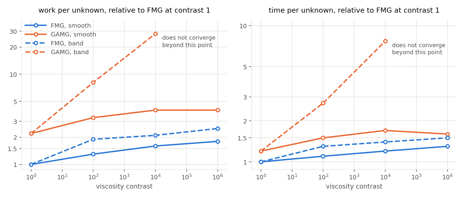
Cost against viscosity contrast for the two viscosity distributions, at 11 727 unknowns. FMG is almost indifferent to the change. GAMG is not: on the band its cost climbs with the contrast, and at 106 it does not converge at all — 20 000 multigrid cycles per velocity solve without reaching the tolerance. This is not an artefact of an under-resolved band. At this resolution the band spans about six cells, and resolving it better does not rescue GAMG: at four and sixteen times the cell count, GAMG’s disadvantage against FMG on the band grows from 5.5 to 7.9 to 8.0 times its disadvantage on the smooth problem at the same size.
The geometric hierarchy is indifferent to the coefficients because it never consults them. That is the case for keeping a hierarchy when you can.
Using it
# Build the hierarchy at mesh construction: base + two refinements.
mesh = uw.meshing.UnstructuredSimplexBox(cellSize=0.05, refinement=2)

stokes = uw.systems.Stokes(mesh)
stokes.preconditioner = "auto"        # FMG when a hierarchy exists
stokes.solve()

print(len(mesh.dm_hierarchy))         # how many levels there are
print(stokes.preconditioner_settings) # what was applied
print(stokes.pc_fallbacks)            # anything declined, and why
If a solve is slow and the mesh has no hierarchy, this is the first thing to
change: rebuild it with refinement rather than at a fine cellSize, and the
same resolution arrives with the coarse levels attached. Note that cellSize
then sets the coarsest mesh, and each refinement halves it — so cellSize=0.05
with refinement=2 resolves like cellSize=0.0125.