Underworld3

The most recent version of Underworld (v3), is a ground-up rewrite of our widely-used geodynamics modelling code. I don't think there is a single line of code carried forward from v2. Underworld3 does share many ideas with Underworld2: it is a finite element code in which particle swarms and mesh variables have equal standing, with a python front end and a parallel-optimised (PETSc) back end, with rich symbolic algebra capabilities to help set up the mathematics of your model (this time we are using sympy), and full integration with the Jupyter notebook system for designing and analysing problems.

We say that Underworld3 is mathematically self-describing because every data object has a symbolic (sympy) equivalent, all the equation systems retain their symbolic representation throughout the problem assembly and, as a result, when you have finished building your problem, you can ask to see the mathematical representation of the numerical implementation. The symbolic representation that Underworld uses makes it easy to evaluate model derivatives for non-linear problems and optimisations, and it also means that you can view, check, simplify and re-use those derivatives in a mathematical form later in your scripts.

There is very little performance penalty for providing this mathematical introspection because sympy compiles PETSc-compatible C-functions when they are needed. This extra compilation step is offset by the fact that sympy can simplify expressions, combine terms, and eliminate common identities before compilation (this is particularly useful when computing Jacobians).

How does this look in practice ?

Underworld3 provides python templates for a number of equations such as Stokes or Advection-Diffusion, which do two things:

• Set up the general equation-solving infrastructure for the equation you want to solve, validate the variables (define new variables if they are not provided), add auxiliary solvers where coupled sub-equations are part of the problem, and so on. For example, in advection-diffusion problems, the advection part of the solver has a number of sub-components that require orchestration behind-the-scenes.
• Provide a number of hooks that the template requires you to fill out in order to solve the problem. For example, Stokes requires an expression for the body force, the addition of a constitutive model and its material properties, boundary conditions which may be functions of the unknowns.

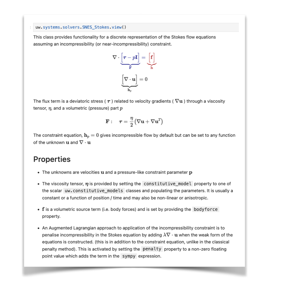
The solver classes are self-describing. We can view() the class description before created a solver to see if this is what we need:

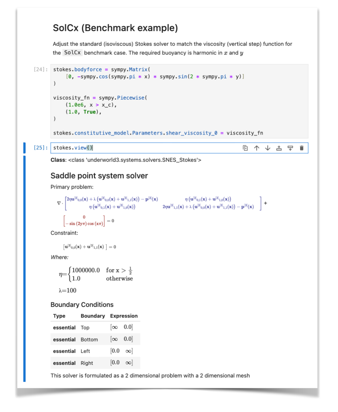
In a notebook, the Stokes problem is set up with some simple python code, most of which is to provide suitable expressions for the constitutive parameters, boundary conditions and the right-hand-side. When we view the solver object (rather than the class), it shows the mathematical description of how it has been set up. This is the superficial description, if you want to find out what the Jacobians look like, you can dig a bit deeper and find out !

Why do I need the mathematical description, really ?

With Underworld3 we haven't attempted to hide away all the mathematical complexity that you need to know to do a good job of numerical modelling, so why do we think it is helpful to add this level of "self-description" ?

The use of sympy is to let the equations simplify and combine terms (for example, it automatically degenerates a viscoelastic problem to a viscous one if the elastic moduli vanish) and we think that you should be aware of what it is doing.

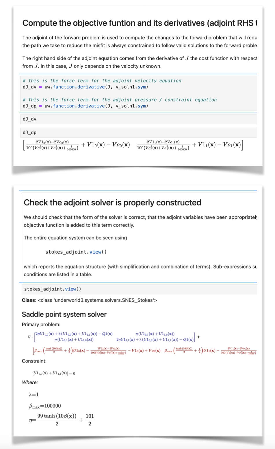
Here is an example: in this optimisation problem, we need to compute derivatives of the objective function (sorry, "funtion" !) and we also clone the original solver with new variables. The validation might just be a visual inspection of the solver, but you can also grab the terms individually and simplify or substitute into them to check they are correct.

How do I get started ?

You can also check the Underworld3 Quickstart guide to browse example notebooks and see how to install the code. Before you install anything, though, you might like to try running the example notebooks on mybinder.org.

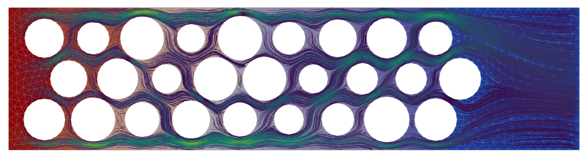
Feature image: Underworld3 uses unstructured meshes supplied by gmsh or any other tool supported by PETSc. In this image we see flow driven from the left boundary around a series of obstacles visualised by streamlines. The intense colours appear where the flow is strongest which is also where the gaps between obstacles line up. There is an emergent pressure gradient displayed in the background shading.